CHEM 548: Materials Chemistry
Lecture 21: Superconductors
Reading: Woodward, Karen, Evans, and Vogt, Solid State Materials Chemistry
Ch. 12; Ch. 9 §§9.2–9.3
Chapter 12: Superconductors
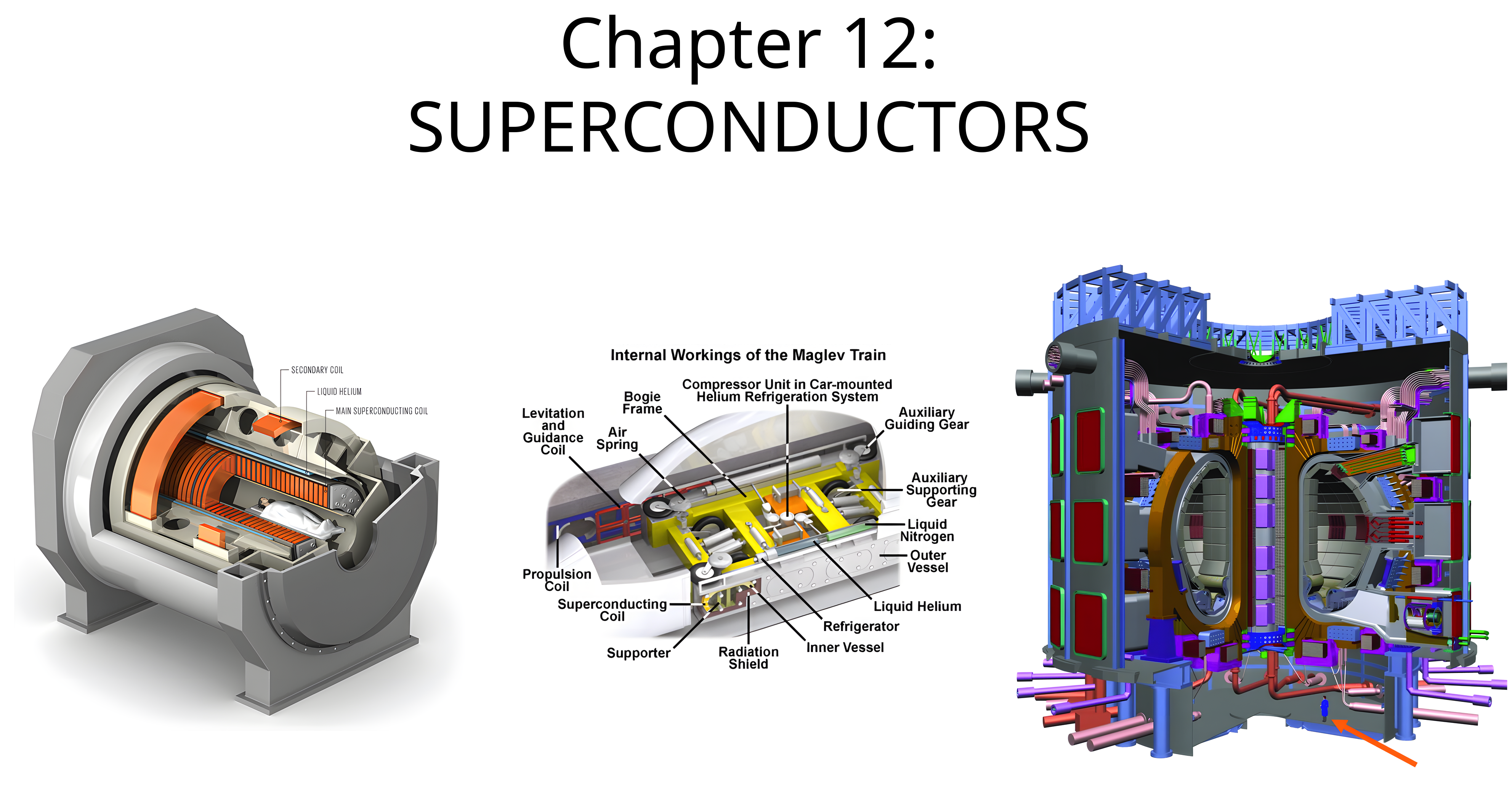
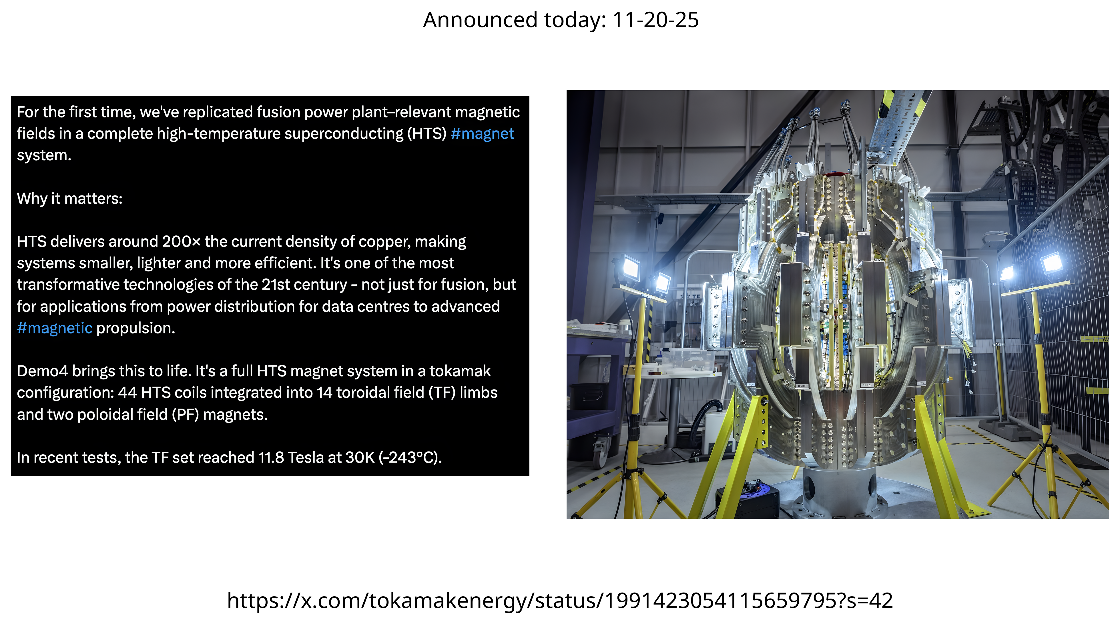
Superconducting Magnets in the News
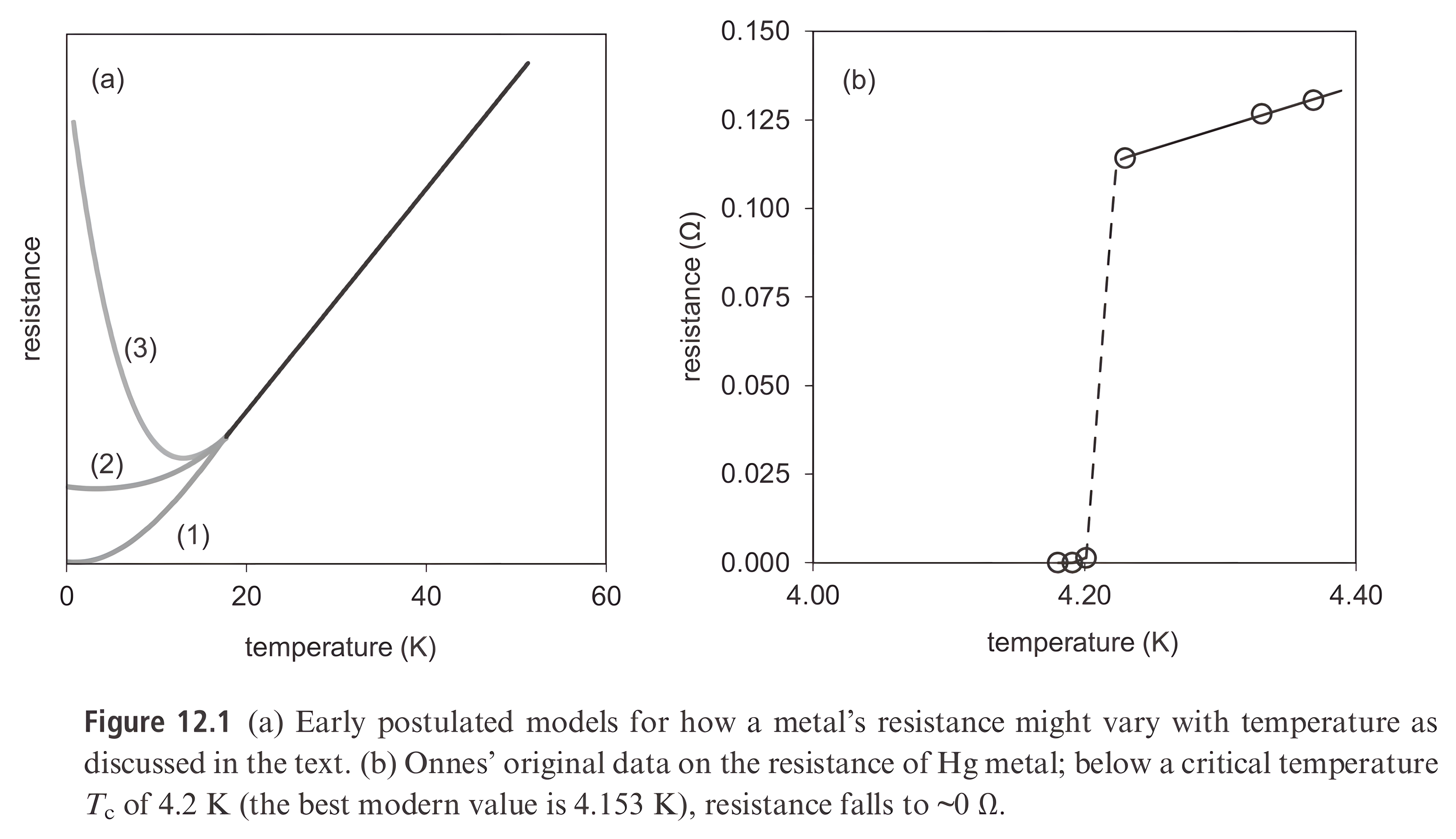
The Discovery of Superconductivity
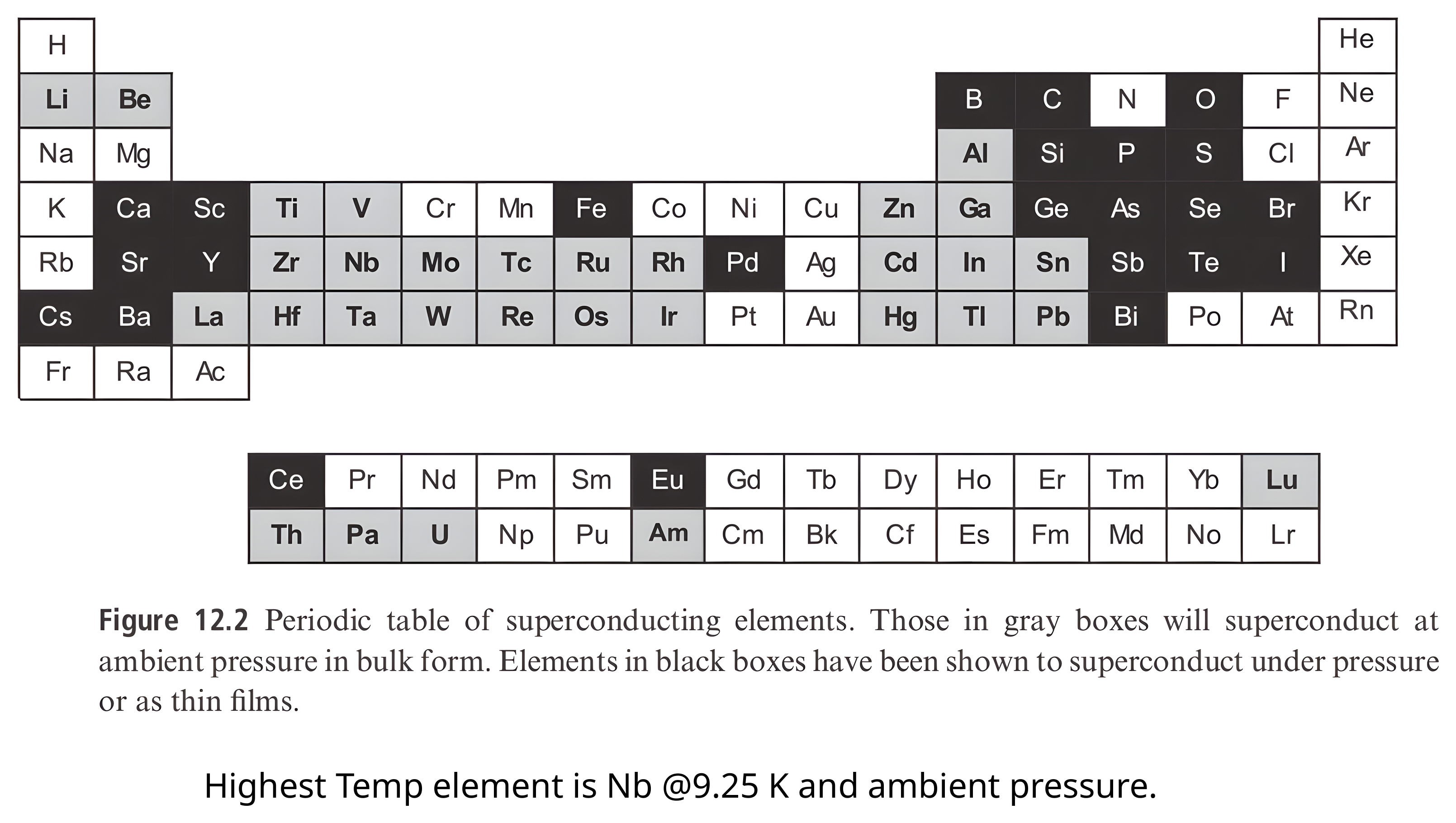
Superconducting Elements
Superconductors and Their Critical Temperatures
| Material | Tc (K) | Comment |
|---|---|---|
| Rh | 0.0003 | Lowest Tc of any superconducting element |
| Hg | 4.153 | First superconductor discovered in 1911 |
| Pb | 7.2 | Highest-Tc type-I superconducting element |
| Nb | 9.25 | Highest-Tc type-II superconducting element |
| Li | 0.004/20 | Ambient/~30 GPa |
| Ca | 21–25 | Highest-Tc element ~220 GPa |
| Nb₃Sn | 18 | High-Tc intermetallic |
| Nb₃Ge | 23.2 | Highest-Tc intermetallic |
| NbO | 1.5 | First oxide superconductor, 1933 |
| SrTiO₃₋δ | 0.3 | First perovskite superconductor |
| BaPb₁₋ₓBiₓO₃ | 13 | First high-temperature superconductor of 1970s |
| Ba₀.₆K₀.₄BiO₃ | 34 | Highest Tc of BaBiO₃-related systems |
| La₁.₈₅Ba₀.₁₅CuO₄ | 30 | First cuprate superconductor, 1986 |
| La₁.₈₅Sr₀.₁₅CuO₄ or La₂CuO₄.₀₈ | 38 | Highest-Tc “214” cuprate superconductor |
| YBa₂Cu₃O₇ | 93 | First >77 K (N₂ boiling point) superconductor, 1987 |
| HgBa₂Ca₂Cu₃O₈₊ₓ | 134/164 | Highest-Tc cuprate at ambient/elevated pressure |
| Ba₁₋ₓSrₓCuO₂ | 90 | Infinite-layer cuprate |
| Ca₁₋ₓSrₓCuO₂ | 110 | Highest-Tc ternary infinite-layer cuprate |
Applied Magnetic Field
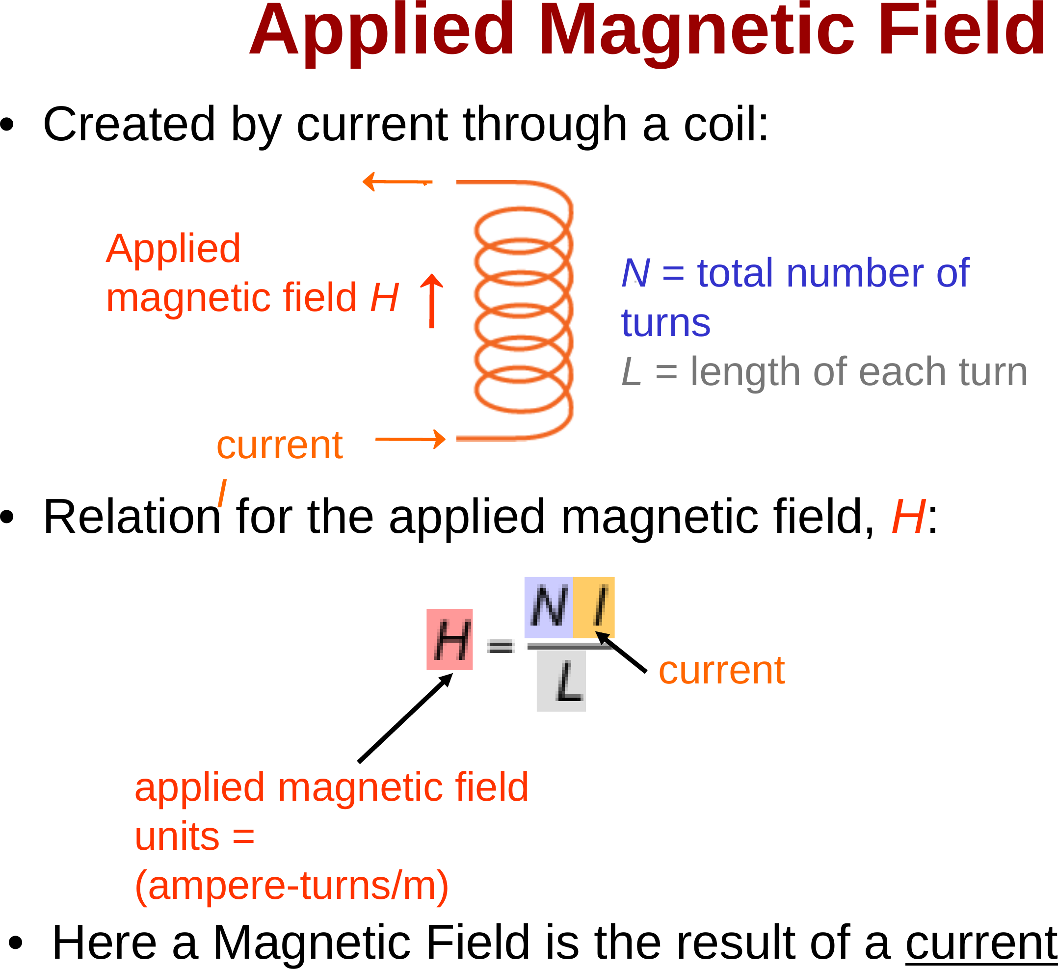
Response to a Magnetic Field
Magnetic induction results in the material
$B_0 = \mu_0 H$ $B = \mu H$ $\mu_r = \mu/\mu_0$ $B = \mu_0 H + \mu_0 M$ $M = (\mu_r - 1)H$
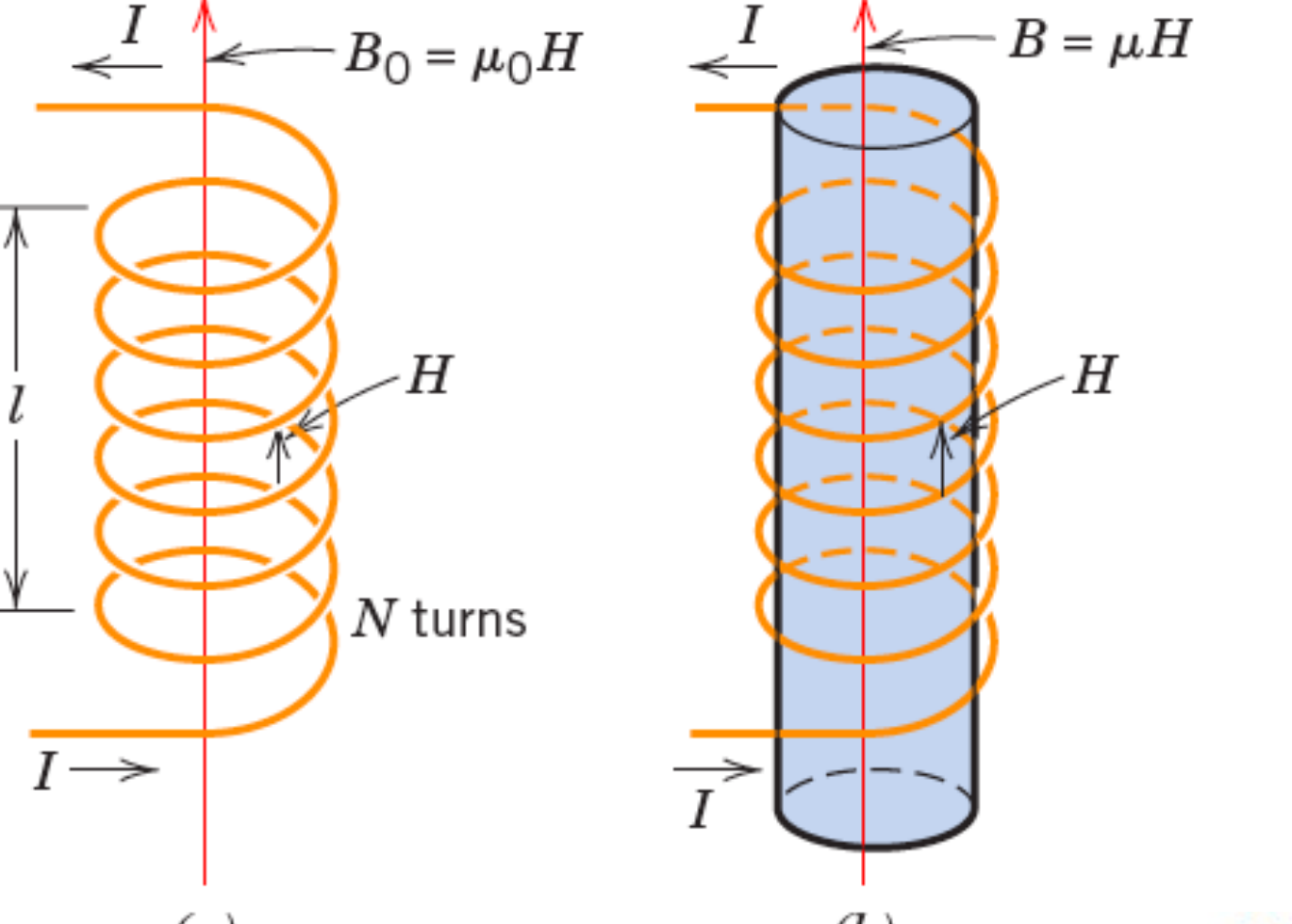
Contribution to the field due to magnetization of the solid
| SI Units | |||
|---|---|---|---|
| Quantity | Symbol | Derived | Primary |
| Magnetic induction (flux density) | B | tesla (Wb/m2)a | kg/s-C |
| Permeability of a vacuum | μ0 | henry/mb | kg-m/C2 |
| Magnetic field strength | H | amp-turn/m | C/m-s |
| Magnetization | M (SI) I (cgs–emu) | amp-turn/m | C/m-s |
Response to a Magnetic Field
Magnetic susceptibility, χ (dimensionless)
χ measures the material response relative to a vacuum.
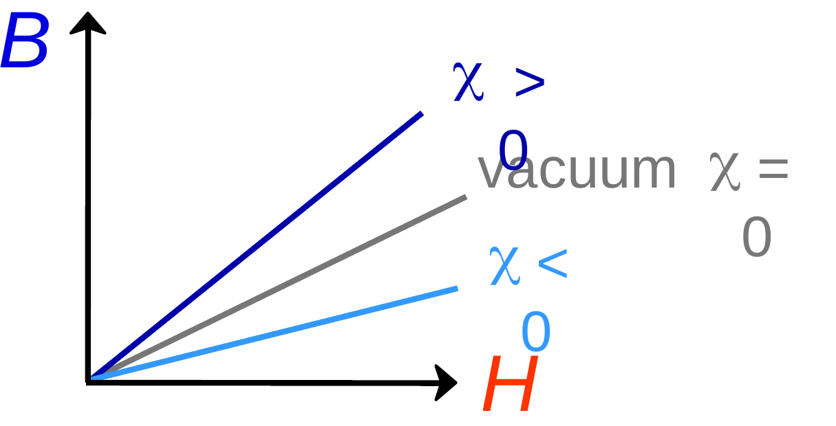
$B = \mu_0(H+M) = \mu_0(1+\chi_m)H = \mu H$
$M = \chi_m H$ $\chi_m = \mu_r - 1$
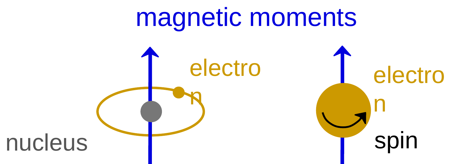
Origins of Magnetic Moments
Electrons produce magnetic moments:
Labels: magnetic moments · electron · nucleus · electron · spin
Net magnetic moment:
--Sum of moments from all electrons.
Three types of response...
Chapter 20 - 39
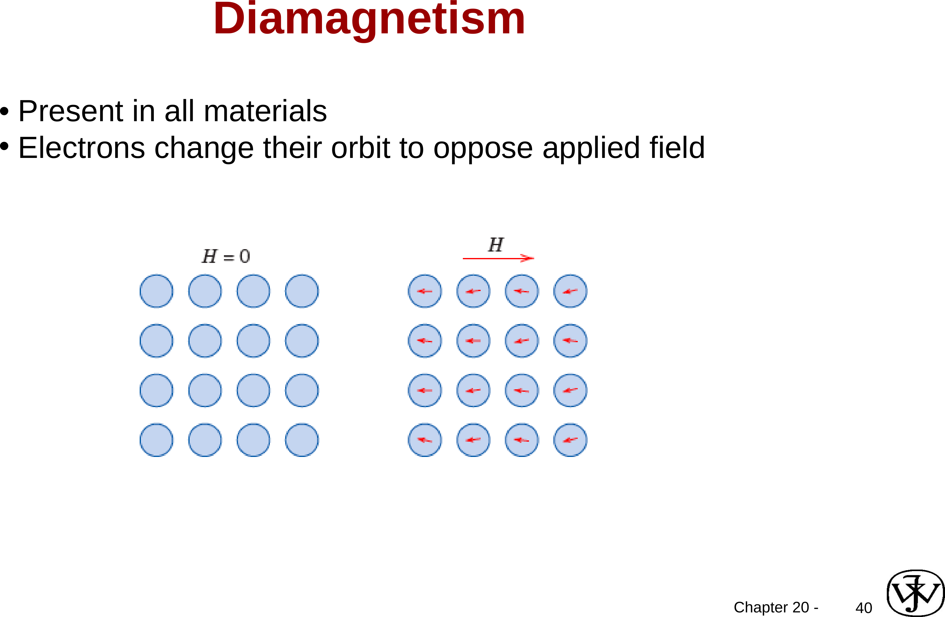
Diamagnetism
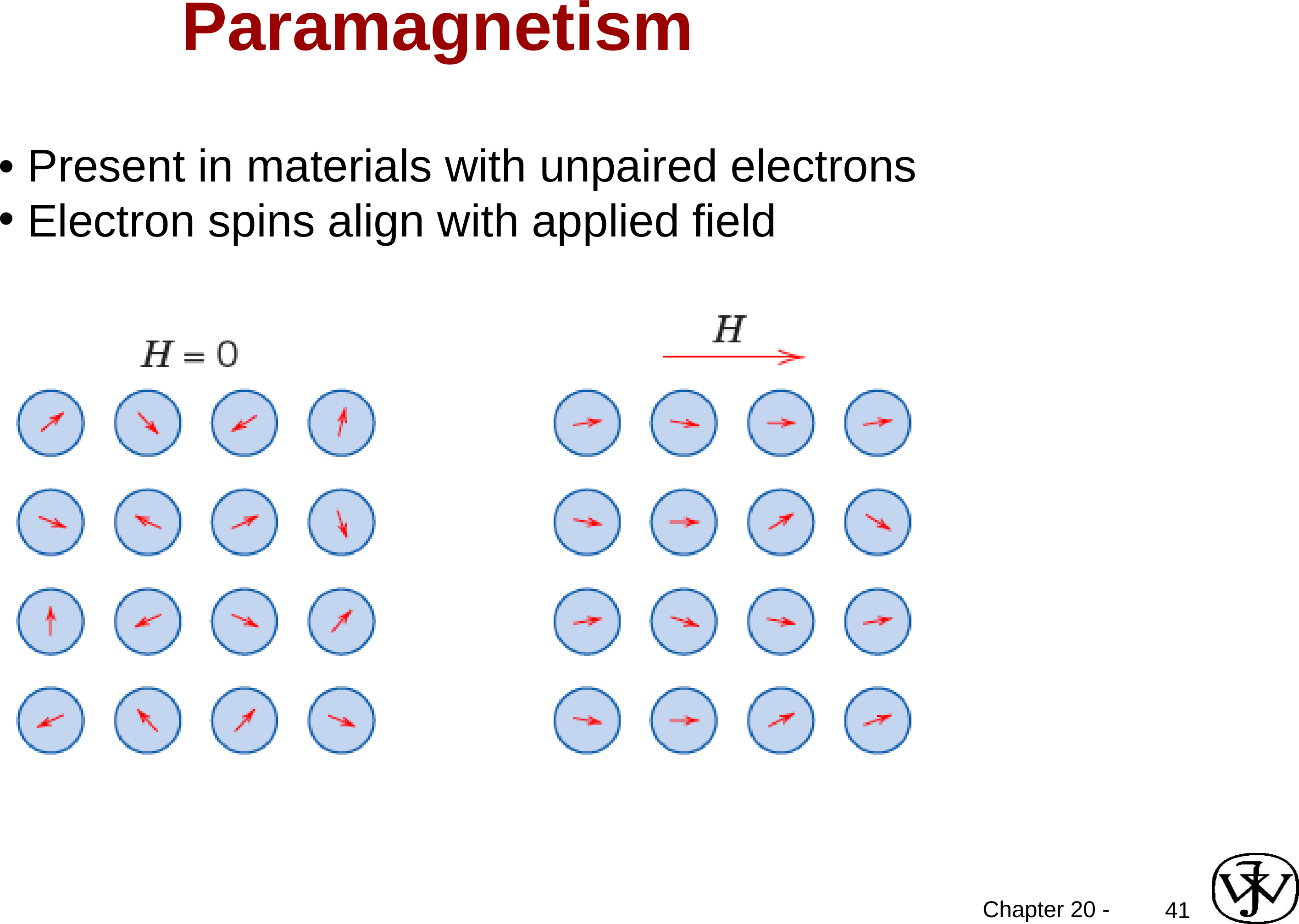
Paramagnetism
Ferromagnetism
Spins couple and align with no applied field
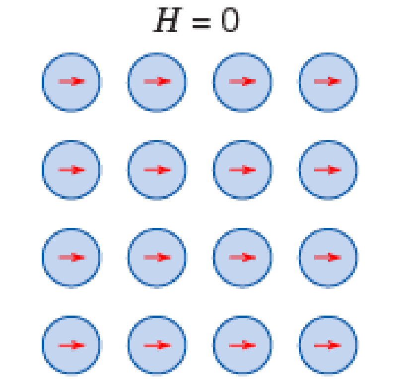
Table 14.1. Magnetic Constants of Some Materials at Room Temperature.
| Material | χ (SI) unitless | χ (cgs) unitless | μ unitless | Type of magnetism |
|---|---|---|---|---|
| Low carbon steel | ≈5 × 10³ | 3.98 × 10² | 5 × 10³ | Ferromagnetic |
| Fe–3%Si (grain-oriented) | 4 × 10⁴ | 3.18 × 10³ | 4 × 10⁴ | |
| Ni–Fe–Mo (supermalloy) | 106 | 7.96 × 10⁴ | 106 |
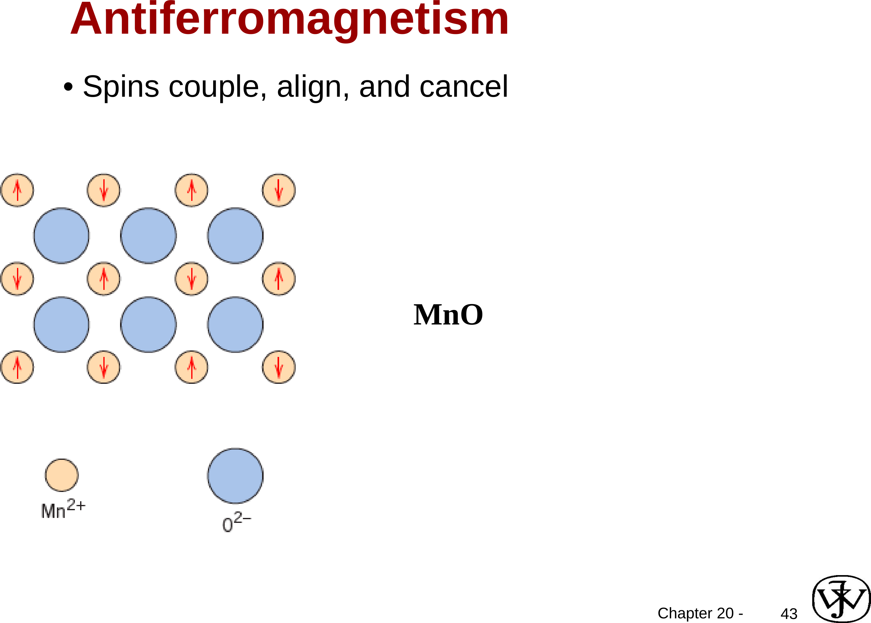
Antiferromagnetism
Magnetic Constants of Some Materials
Table 14.1. Magnetic Constants of Some Materials at Room Temperature.
| Material | χ (SI) unitless | χ (cgs) unitless | μ unitless | Type of magnetism |
|---|---|---|---|---|
| Bi | −165 × 10−6 | −13.13 × 10⁻⁶ | 0.99983 | Diamagnetic |
| Ge | −71.1 × 10⁻⁶ | −5.66 × 10⁻⁶ | 0.99992 | |
| Au | −34.4 × 10⁻⁶ | −2.74 × 10⁻⁶ | 0.99996 | |
| Ag | −23.8 × 10⁻⁶ | −1.90 × 10⁻⁶ | 0.99997 | |
| Be | −23.2 × 10⁻⁶ | −1.85 × 10⁻⁶ | 0.99998 | |
| Cu | −9.7 × 10⁻⁶ | −0.77 × 10⁻⁶ | 0.99999 | |
| Water | −9.14 × 10⁻⁶ | −0.73 × 10⁻⁶ | 0.99999 | |
| Si | −4.1 × 10⁻⁶ | −0.32 × 10⁻⁶ | 0.99999 | |
| Superconductorsa | −1.0 | ~−8 × 10⁻² | 0 | |
| β-Sn | +2.4 × 10⁻⁶ | +0.19 × 10⁻⁶ | 1 | Paramagnetic |
| Al | +20.7 × 10⁻⁶ | +1.65 × 10⁻⁶ | 1.00002 | |
| W | +77.7 × 10⁻⁶ | +6.18 × 10⁻⁶ | 1.00008 | |
| Pt | +264.4 × 10⁻⁶ | +21.04 × 10⁻⁶ | 1.00026 | |
| Low carbon steel | ≈5 × 10³ | 3.98 × 10² | 5 × 10³ | Ferromagnetic |
| Fe–3%Si (grain-oriented) | 4 × 10⁴ | 3.18 × 10³ | 4 × 10⁴ | |
| Ni–Fe–Mo (supermalloy) | 106 | 7.96 × 10⁴ | 106 |
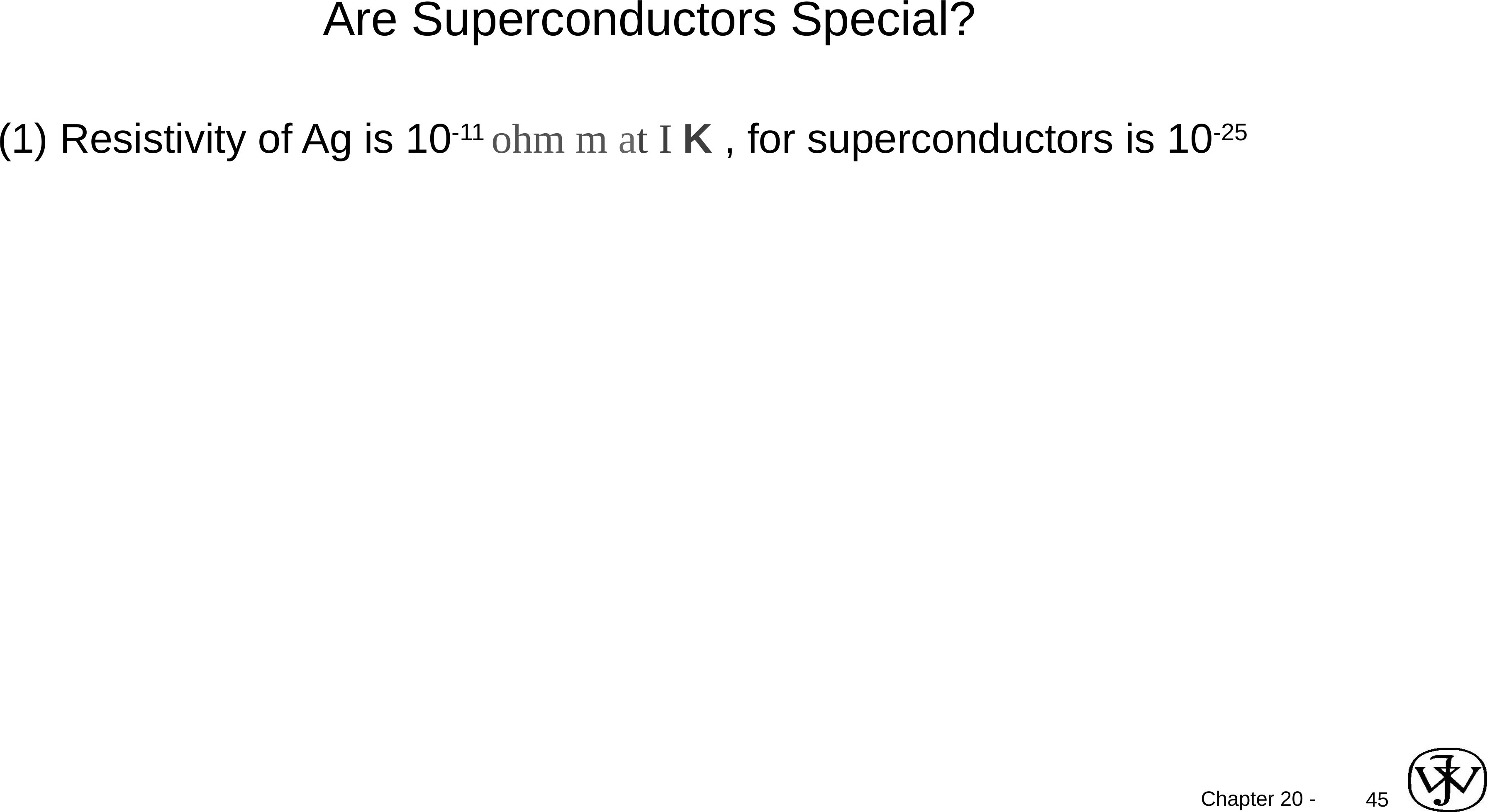
Are Superconductors Special?
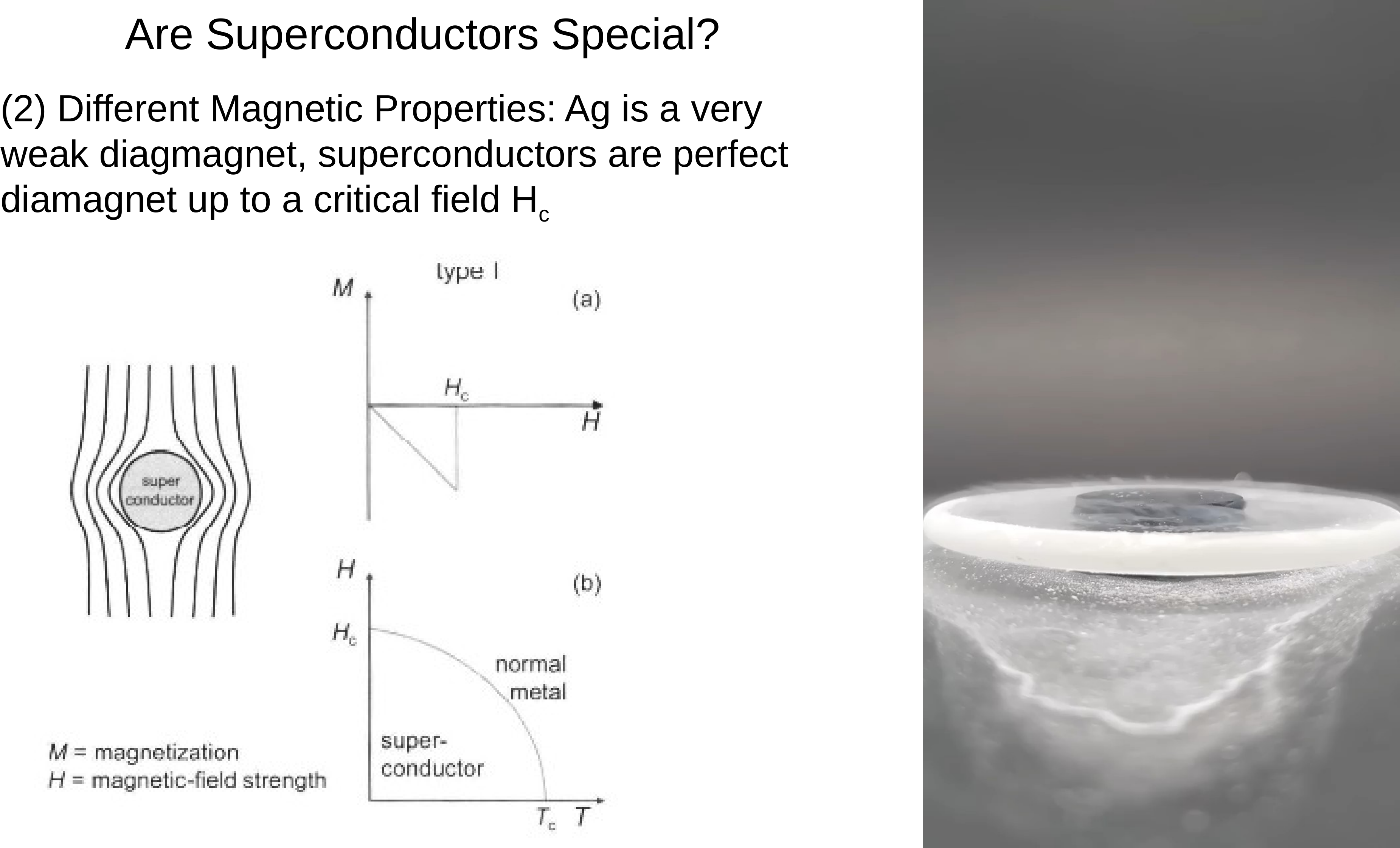
The Meissner Effect
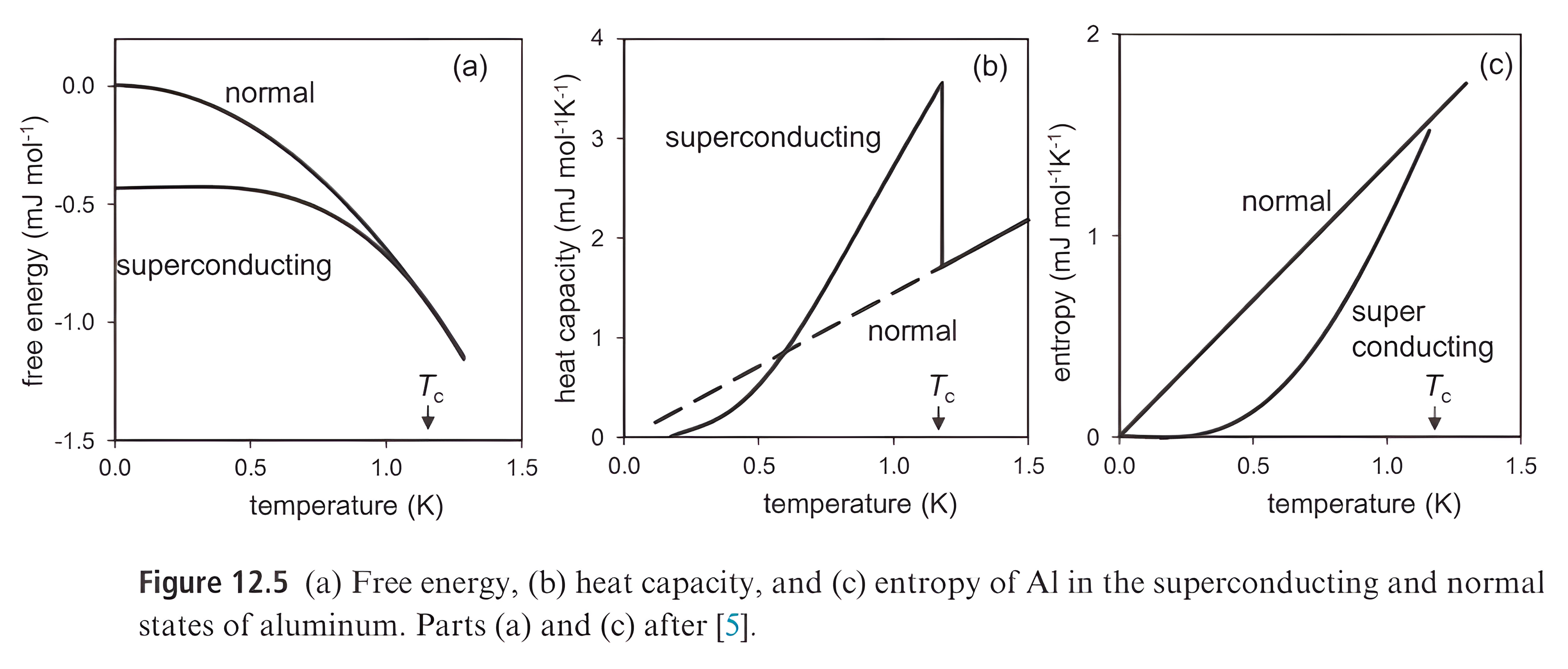
A Second-Order Transition
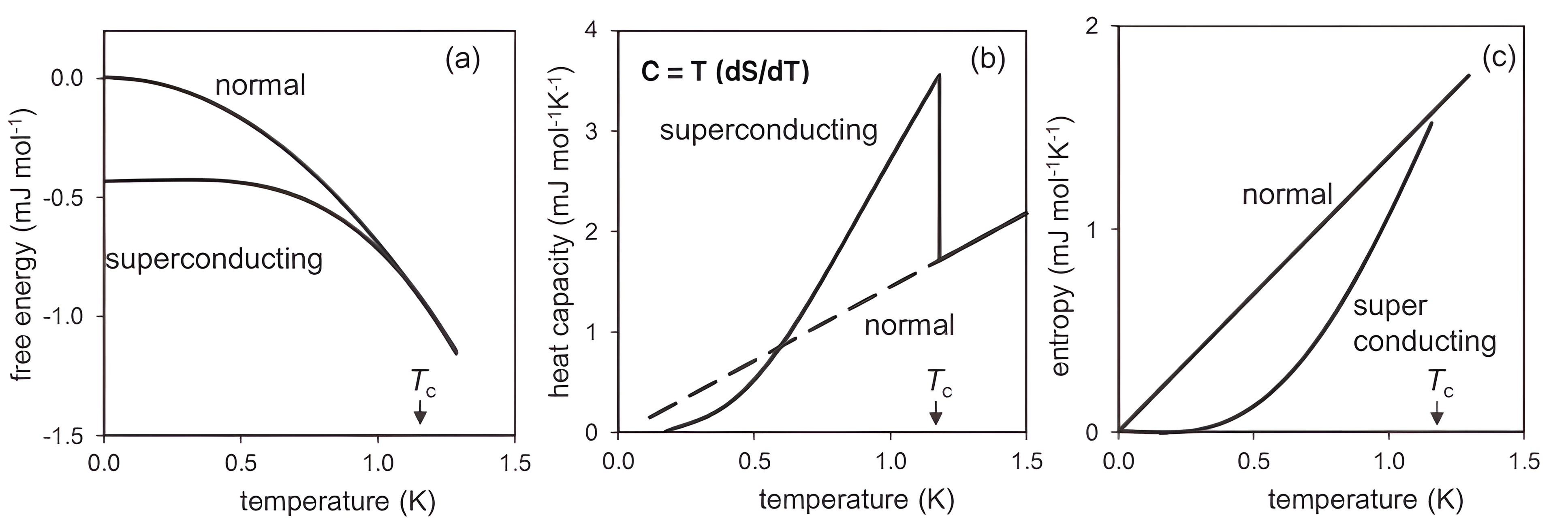
(3) Thermodynamic Analysis reviews Tc is associated with a 2nd order transition
free energy (mJ mol−1) · heat capacity (mJ mol−1K−1) · entropy (mJ mol−1K−1) · temperature (K) · C = T (dS/dT) · superconducting · normal · super conducting
Figure 12.5 (a) Free energy, (b) heat capacity, and (c) entropy of Al in the superconducting and normal states of aluminum. Parts (a) and (c) after [5].
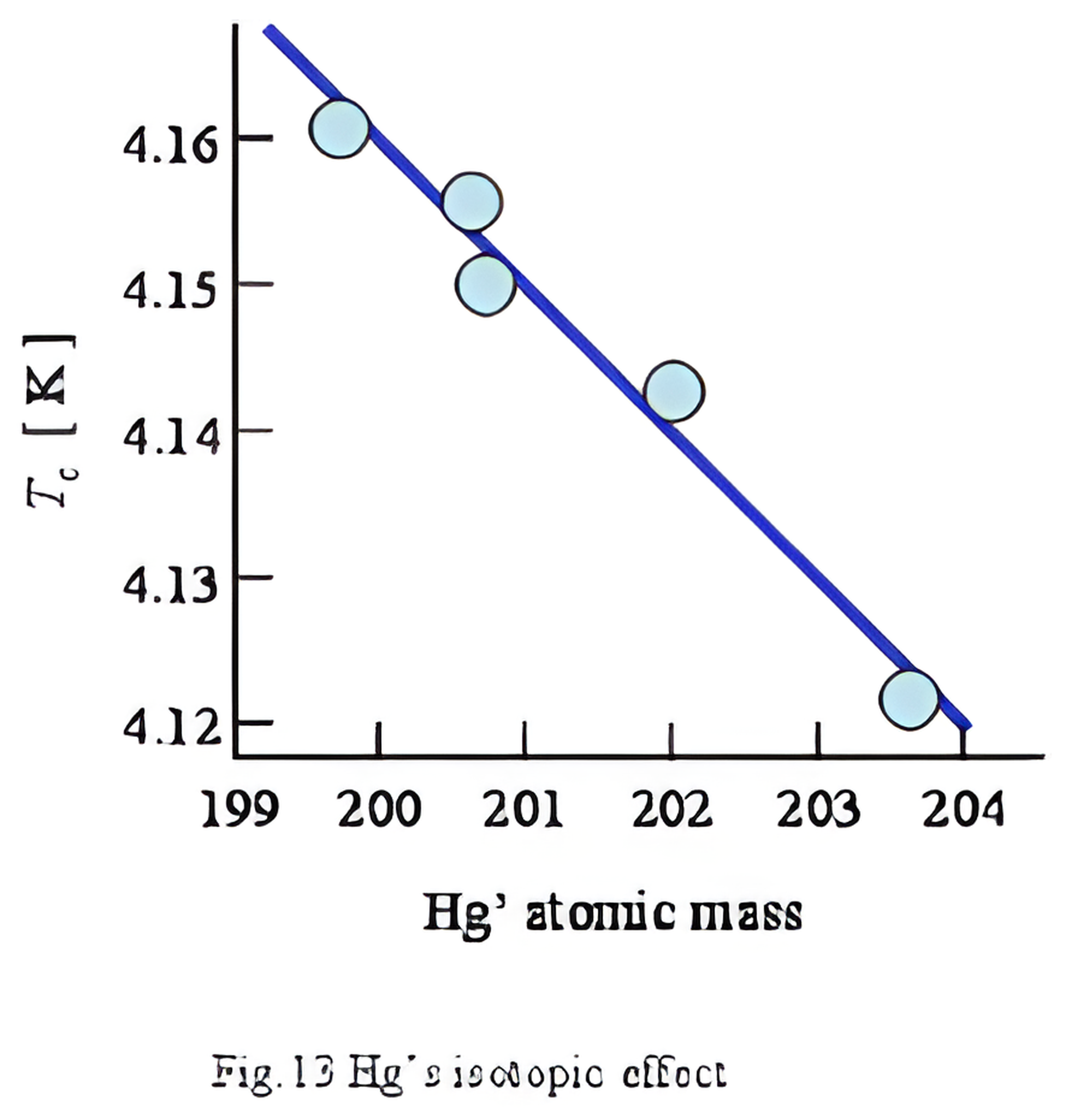
The Isotope Effect
BCS Theory (1957)
PHYSICAL REVIEWVOLUME 108, NUMBER 5DECEMBER 1, 1957
Theory of Superconductivity*
J. BARDEEN, L. N. COOPER,† AND J. R. SCHRIEFFER‡
Department of Physics, University of Illinois, Urbana, Illinois
(Received July 8, 1957)
A theory of superconductivity is presented, based on the fact that the interaction between electrons resulting from virtual exchange of phonons is attractive when the energy difference between the electrons states involved is less than the phonon energy, $\hbar\omega$. It is favorable to form a superconducting phase when this attractive interaction dominates the repulsive screened Coulomb interaction. The normal phase is described by the Bloch individual-particle model. The ground state of a superconductor, formed from a linear combination of normal state configurations in which electrons are virtually excited in pairs of opposite spin and momentum, is lower in energy than the normal state by amount proportional to an average $(\hbar\omega)^2$, consistent with the isotope effect. A mutually orthogonal set of excited states in one-to-one correspondence with those of the normal phase is obtained by specifying occupation of certain Bloch states and by using the rest to form a linear combination of virtual pair configurations. The theory yields a second-order phase transition and a Meissner effect in the form suggested by Pippard. Calculated values of specific heats and penetration depths and their temperature variation are in good agreement with experiment. There is an energy gap for individual-particle excitations which decreases from about 3.5kTc at T=0°K to zero at Tc. Tables of matrix elements of single-particle operators between the excited-state superconducting wave functions, useful for perturbation expansions and calculations of transition probabilities, are given.
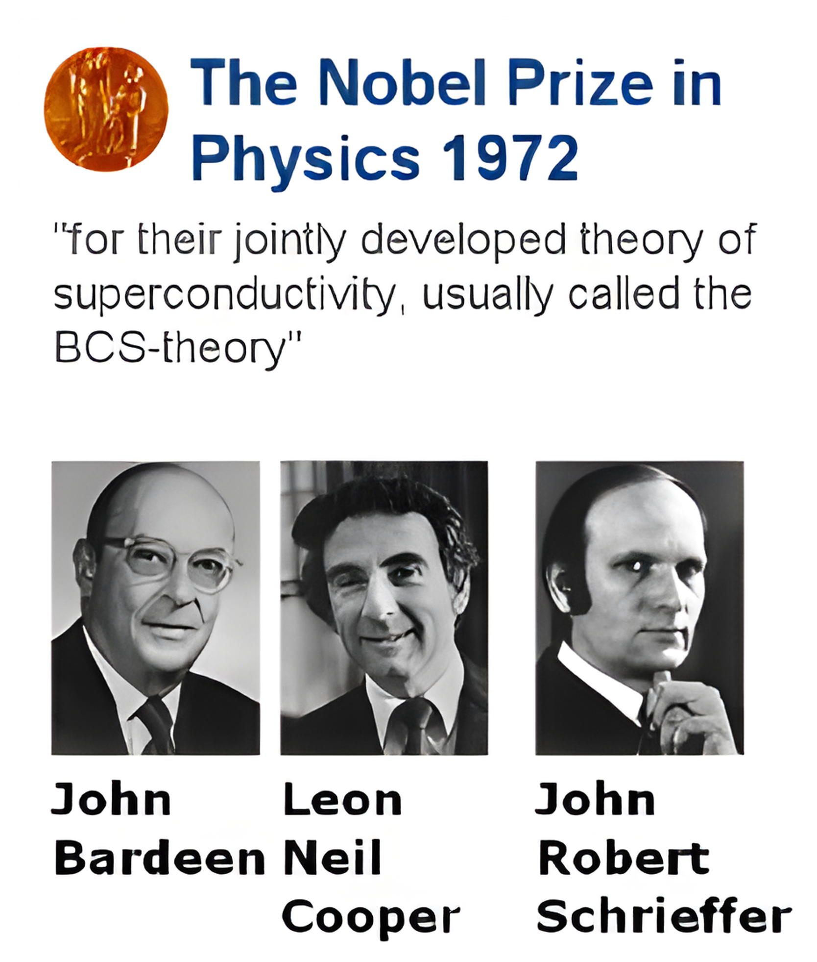
The Nobel Prize in Physics 1972
Electron–Phonon Coupling
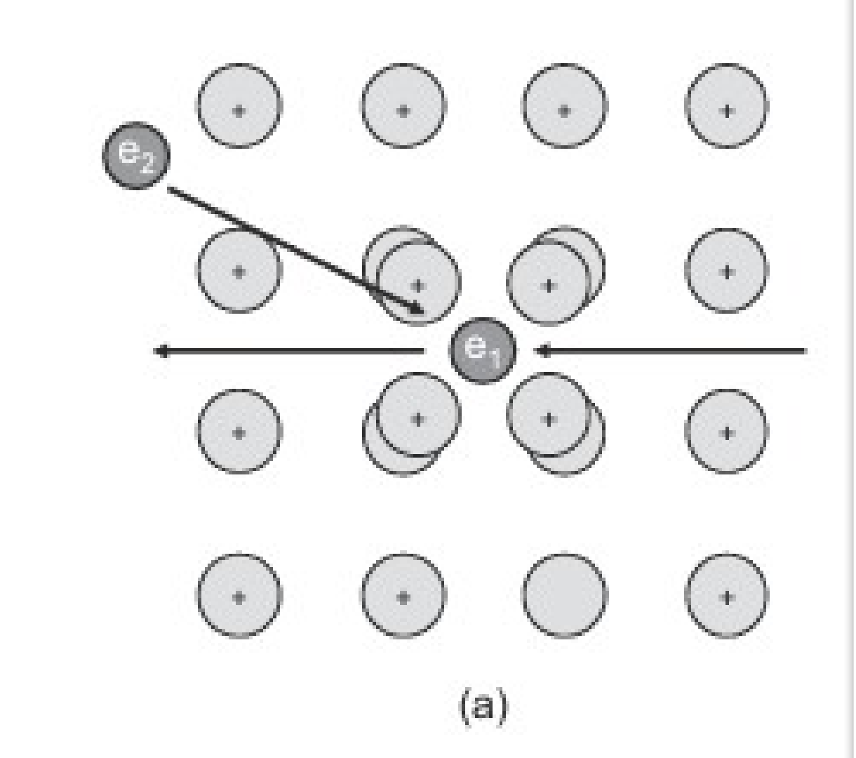
Figure 12.6 (a) Real-space illustration of how electron–phonon coupling in a simple metal system can lead to attractive interaction between two electrons.9 (b) Virtual-phonon exchange behind Cooper-pair formation.
Electron Pairing Distance Estimate
Electron Pairing Distance Estimate
Since electrons move much faster than the heavier metal ions, there is a time delay between the motion of the first electron (which distorts the lattice) and the subsequent attraction of the second electron. To estimate the distance d the first electron has traveled by the time the second is attracted, we use:
- vn: velocity of an electron at the Fermi level
- ω_D: Debye angular frequency, which sets how fast the lattice can respond
The estimated distance is
d = v_F (2π / ω_D)
For aluminum:
- v_F ≈ 2×10⁶ m/s
- ω_D ≈ 5×10¹³ s−1
This gives:
d ≈ 2500 Å
This distance is large compared with atomic spacing, so Coulomb repulsion between the electrons is negligible, especially due to screening by the positively charged metal ions.
Virtual Phonon Exchange
Conservation of momentum leads to the relationships:
$k_1 = k_1' + q$ and $k_2 + q = k_2'$
$(k_1 + k_2) = (k_1' + q) + (k_2' - q)$
$k_1 + k_2 = k_1' + k_2' = k_0$
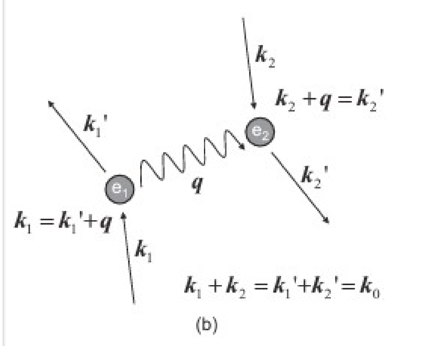
Figure 12.6 (a) Real-space illustration of how electron–phonon coupling in a simple metal system can lead to attractive interaction between two electrons.9 (b) Virtual-phonon exchange behind Cooper-pair formation.
Electron Pairing in $k$-Space
Electron Pairing in k-Space
To form a Cooper pair through phonon exchange, each electron must scatter into a different quantum state. The Pauli exclusion principle limits which states are available: electrons deep below the Fermi energy EF cannot scatter because all nearby states are already occupied. Only electrons close enough to EF have empty states available.
A phonon of energy $\hbar\omega$ can only change an electron’s energy by at most $\hbar\omega$. Therefore, an electron can scatter only if there is an unoccupied state within that energy range. When you combine this with Pauli exclusion, the result is that only electrons within an energy window of order $\hbar\omega$ around EF can participate in pairing.
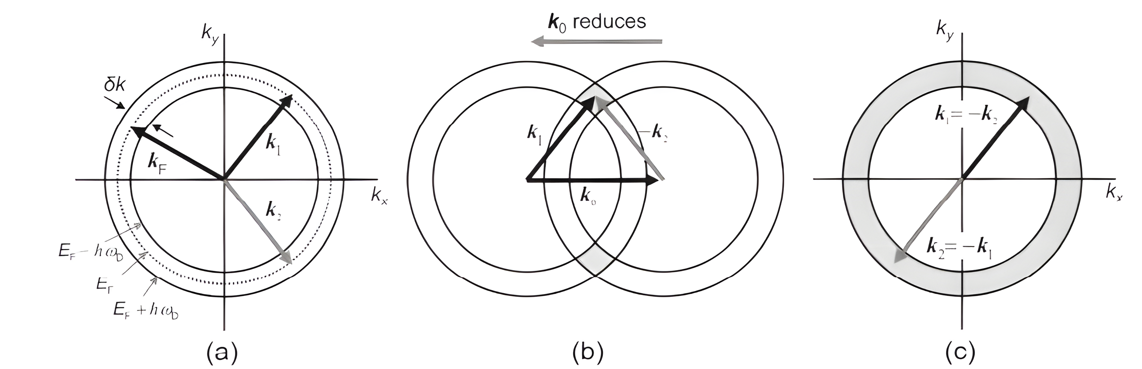
In k-space, this allowed energy window corresponds to a thin shell of states surrounding the Fermi surface, with thickness $\delta k$ determined by $\hbar\omega$. Only electrons whose wave vectors fall within this narrow shell can experience the phonon-mediated attraction, as shown schematically in Figure 12.7.
The Fermi Shell in $k$-Space
$k_0$ reduces
Figure 12.7 (a) A k-space sketch of a spherical shell of states within $\delta k$ of Fermi level $k_\mathrm{F}$. Electrons with arbitrary wave vectors $k_1$ and $k_2$ are shown. The change in $k_1$ on phonon exchange is restricted to a small area determined by $\delta k$. (b) The overall condition of $k_1 + k_2 = k_0$ for virtual phonon exchange can be represented geometrically by two such shells offset by $k_0$. For a given value of $k_0$ the overlap region (shaded) gives the states that can be involved in coupling. The maximum coupling will occur when the two shells overlap such that $k_0 = 0$ and $k_1 = -k_2$.
Why $k_0 = 0$ Maximizes Pairing
Why $k_0 = 0$ gives the most possible pairs
If $k_0 = 0$, then the rule becomes:
$k_2 = -k_1$
That means every state k in the shell automatically has a partner $-k$ that is also in the shell.
This doubles your options: every point on the Fermi surface has a matching point directly opposite it.
So the number of available pair states is maximized.
If $k_0$ is not zero (say, $k_0$ is some nonzero vector), then the partner of $k_1$ is $k_2 = k_0 − k_1$. Many of those points don’t lie in the allowed shell anymore, so the number of available pairs drops.
$s$-Wave Pairing
$k_0 = k_1 + k_2$, so $k_0 = 0$ means:
$k_2 = -k_1$
In other words, the two electrons in a Cooper pair must have equal and opposite momenta.
Because electrons are fermions, their spins must also be opposite for the overall two-electron wavefunction to be allowed. So a Cooper pair consists of states:
$(k, \uparrow)$ and $(-k, \downarrow)$
This is called s-wave pairing, which is the type found in conventional (BCS) superconductors.
Finally, a Cooper pair is not like two electrons locked together in a fixed chemical bond. Instead, it is a dynamic quantum state in which many electrons near the Fermi surface continuously exchange phonons and momentarily form paired states with opposite momenta and opposite spins.
The Superconducting Energy Gap
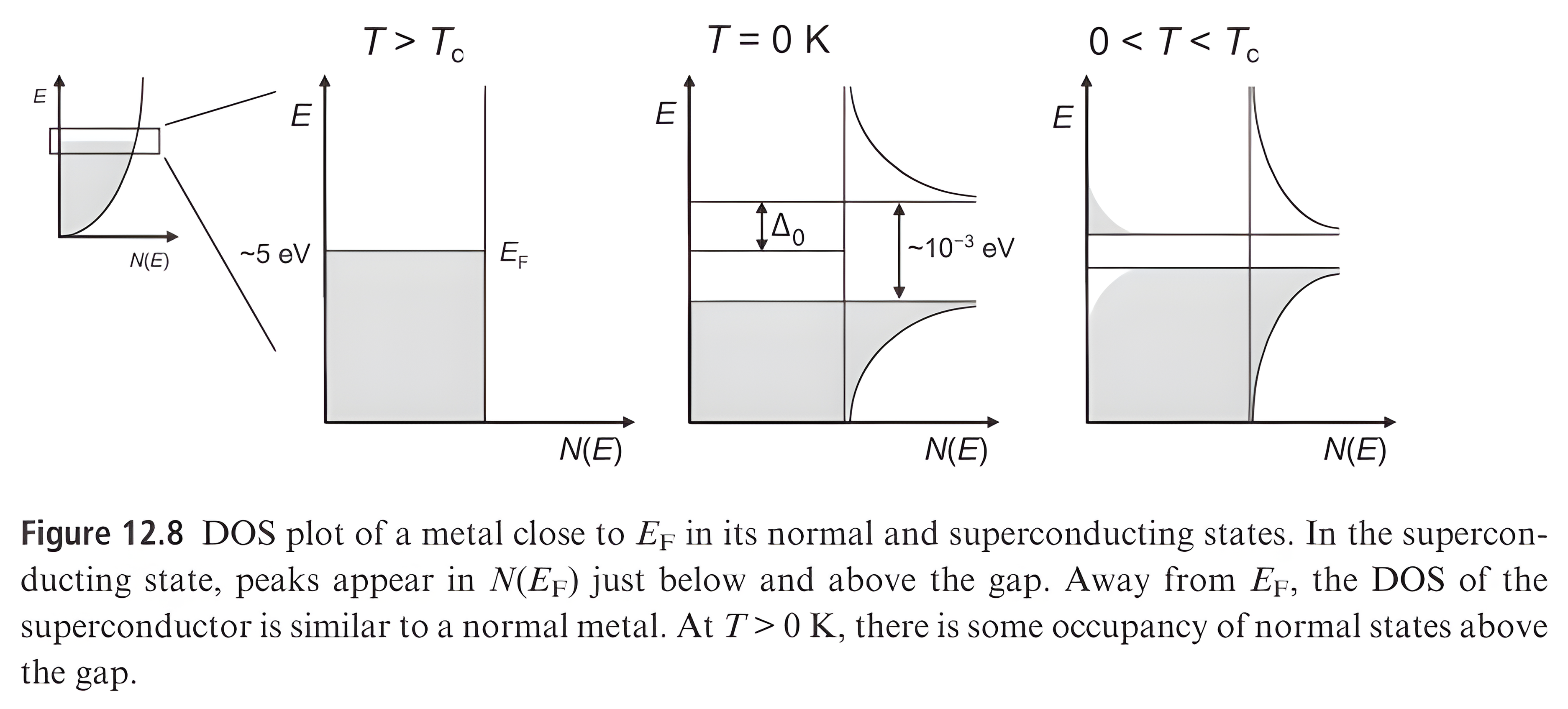
The Second-Order Transition, Revisited
BCS Prediction for the Zero-Temperature Gap and Tc
$$\Delta_0 = \frac{\hbar\omega_D}{\sinh\left[\frac{1}{N(E_F)V}\right]} \approx 2\hbar\omega_D\, e^{-1/(N(E_F)V)}$$
- $N(E_F)$ is the density of states at the Fermi level
- $V$ is the electron–phonon coupling strength
- $\omega_D$ is the Debye frequency
Typical experimental measurements the zero temp energy gap are Δ0 ≈ 5×10⁻⁴ eV
BCS Theory further predicts that $2\Delta_0 = 3.52kT_\mathrm{c}$
Tc = 2Δ0 3.52 kB = 2(5 × 10⁻⁴ eV) 3.52 (8.617 × 10⁻⁵eV/K) ≈ 3.3 K
BCS Evaluated at $T_c$
BCS prediction evaluated at Tc yields:
$$T_\mathrm{c} = 1.14\,\frac{\hbar\omega_\mathrm{D}}{k}\, e^{-1/N(E_\mathrm{F})\cdot V}$$
- The BCS expression for $T_c$ shows that it scales with the Debye frequency $\omega_D$.
This explains the isotope effect and why materials containing light elements (such as MgB₂) can have high $T_c$ due to their high phonon frequencies. - A larger electron–phonon interaction $V$ leads to a higher $T_c$.
This explains why good normal conductors (Cu, Ag, Au), which have weak electron-phonon coupling, are poor superconductors, while poor normal conductors (often oxides with stronger coupling) can be good superconductors.
Why Superconductors Have Zero Resistance
Temperature Milestones for Superconductors
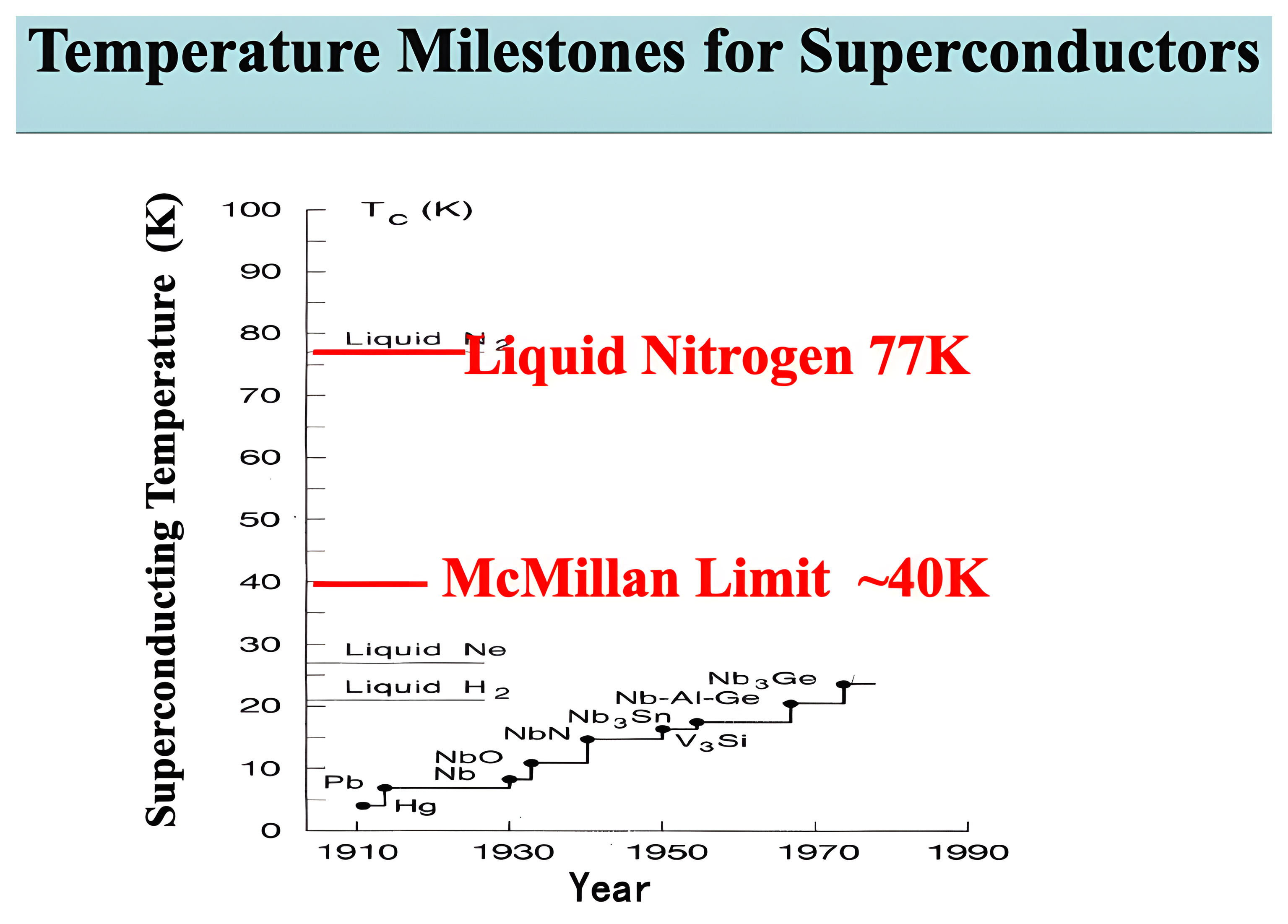
Superconductivity in Copper-Oxide Compounds
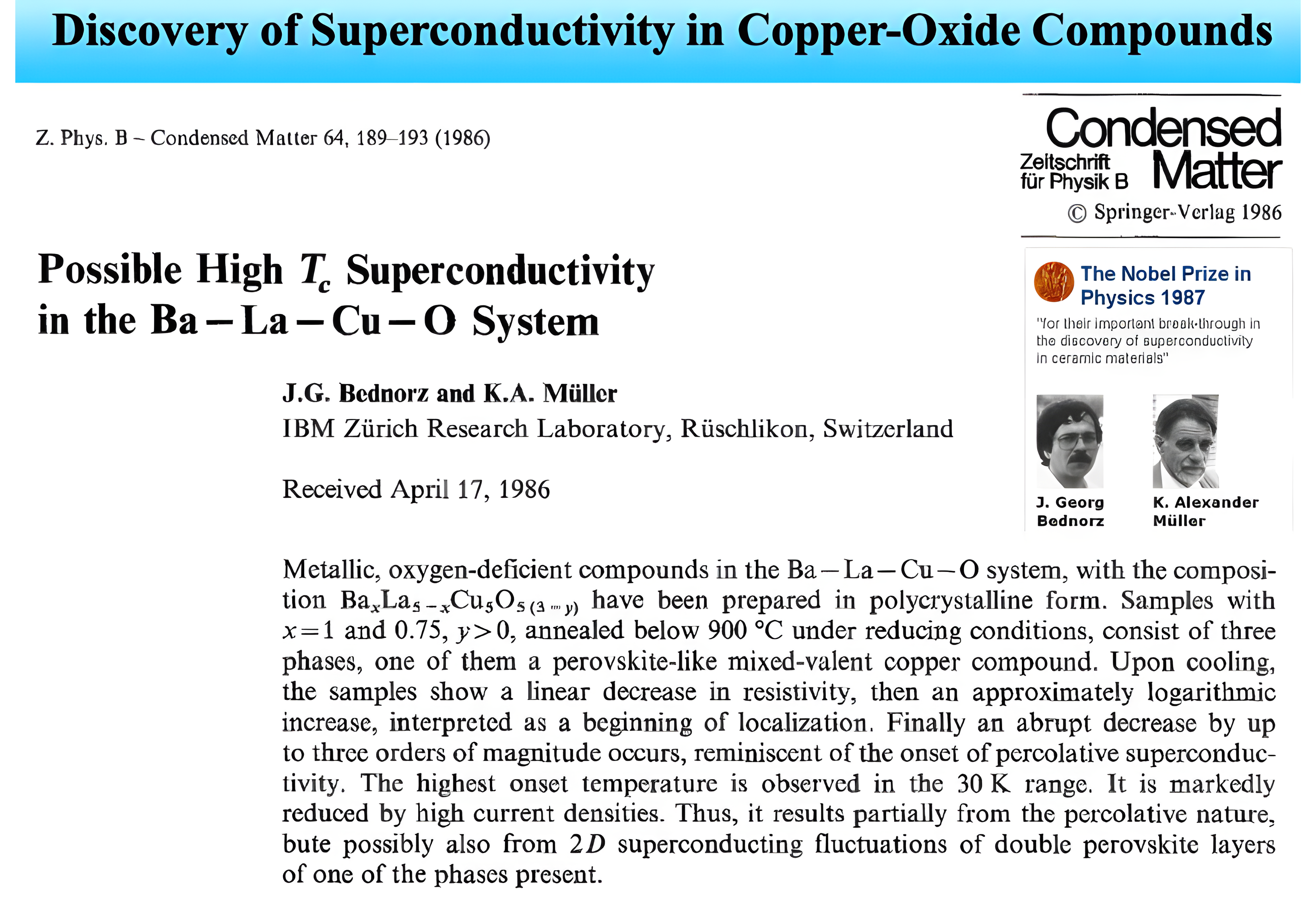
93 K in Y-Ba-Cu-O (1987)
Volume 58, Number 9 Physical Review Letters 2 March 1987
Superconductivity at 93 K in a New Mixed-Phase Y-Ba-Cu-O Compound System
at Ambient Pressure
M. K. Wu, J. R. Ashburn, and C. J. Torng
Department of Physics, University of Alabama, Huntsville, Alabama 35899
and
P. H. Hor, R. L. Meng, L. Gao, Z. J. Huang, Y. Q. Wang, and C. W. Chu(a)
Department of Physics and Space Vacuum Epitaxy Center, University of Houston, Houston, Texas 77004
(Received 6 February 1987: Revised manuscript received 18 February 1987)
A stable and reproducible superconductivity transition between 80 and 93 K has been unambiguously observed both resistively and magnetically in a new Y-Ba-Cu-O compound system at ambient pressure. An estimated upper critical field Hc2(0) between 80 and 180 T was obtained.
Transition Temperatures by Year
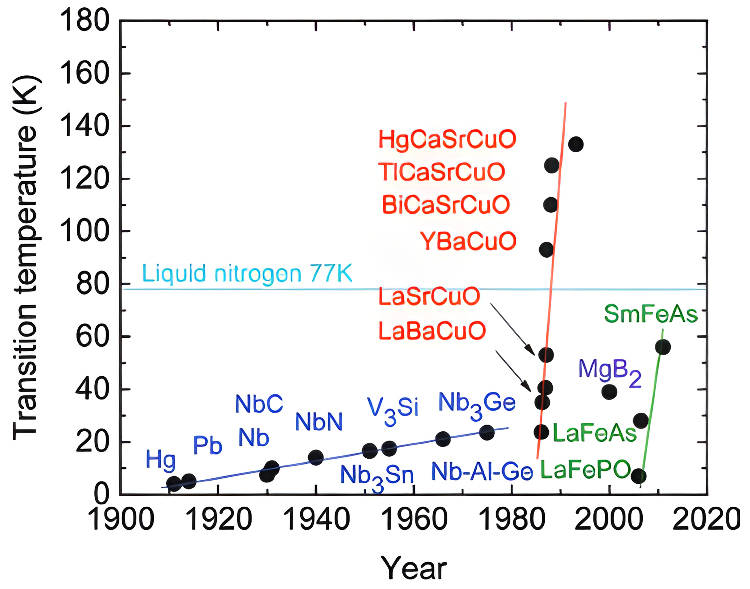
Axes: Transition temperature (K); Year: 1900, 1920, 1940, 1960, 1980, 2000, 2020.
Labelled: Hg · Pb · Nb · NbC · NbN · V₃Si · Nb₃Sn · Nb-Al-Ge · Nb₃Ge · Liquld nitrogen 77K · LaBaCuO · LaSrCuO · YBaCuO · BiCaSrCuO · TlCaSrCuO · HgCaSrCuO · MgB₂ · LaFePO · LaFeAs · SmFeAs.
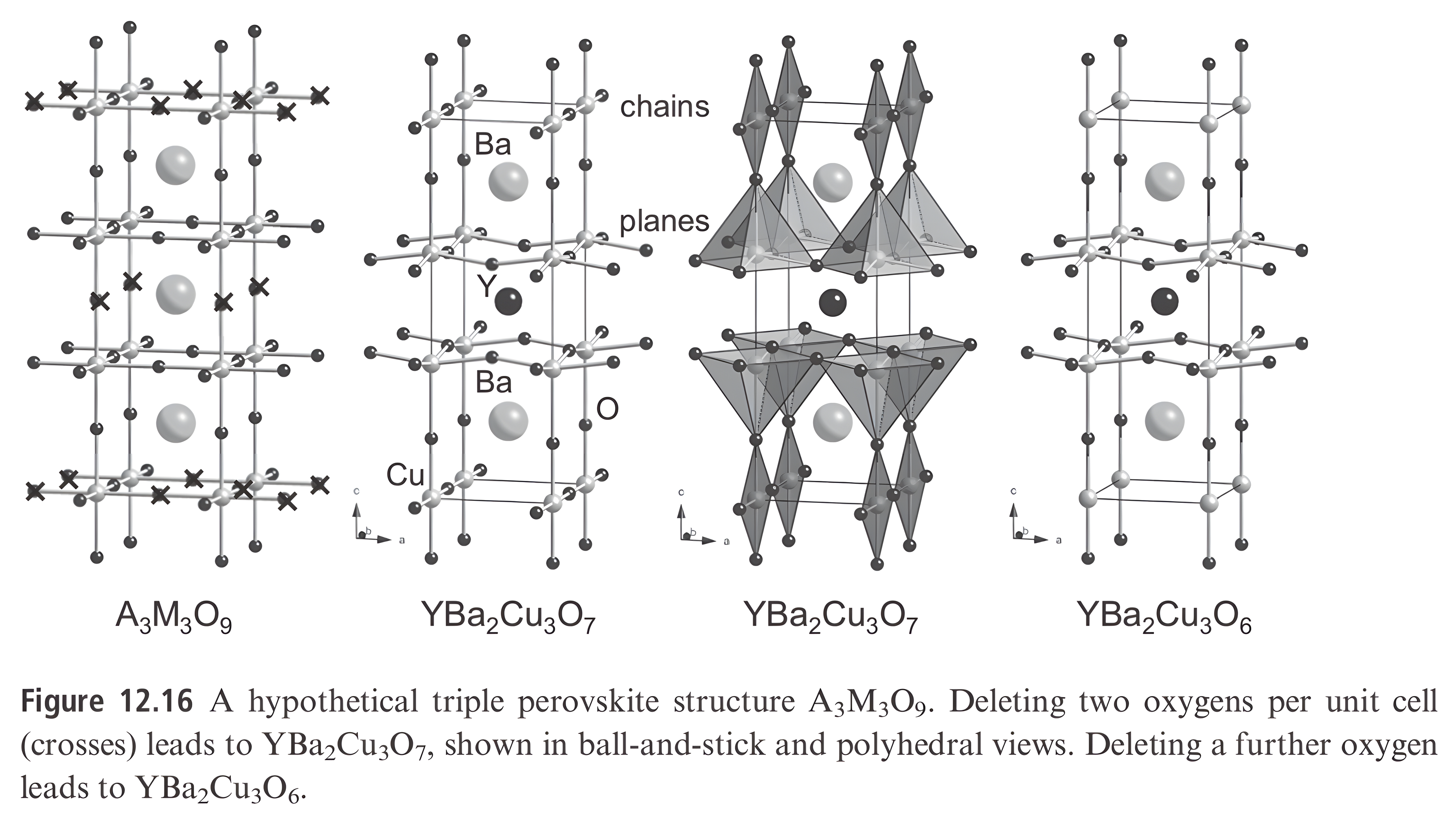
$\mathrm{YBa_2Cu_3O_7}$ from a Triple Perovskite
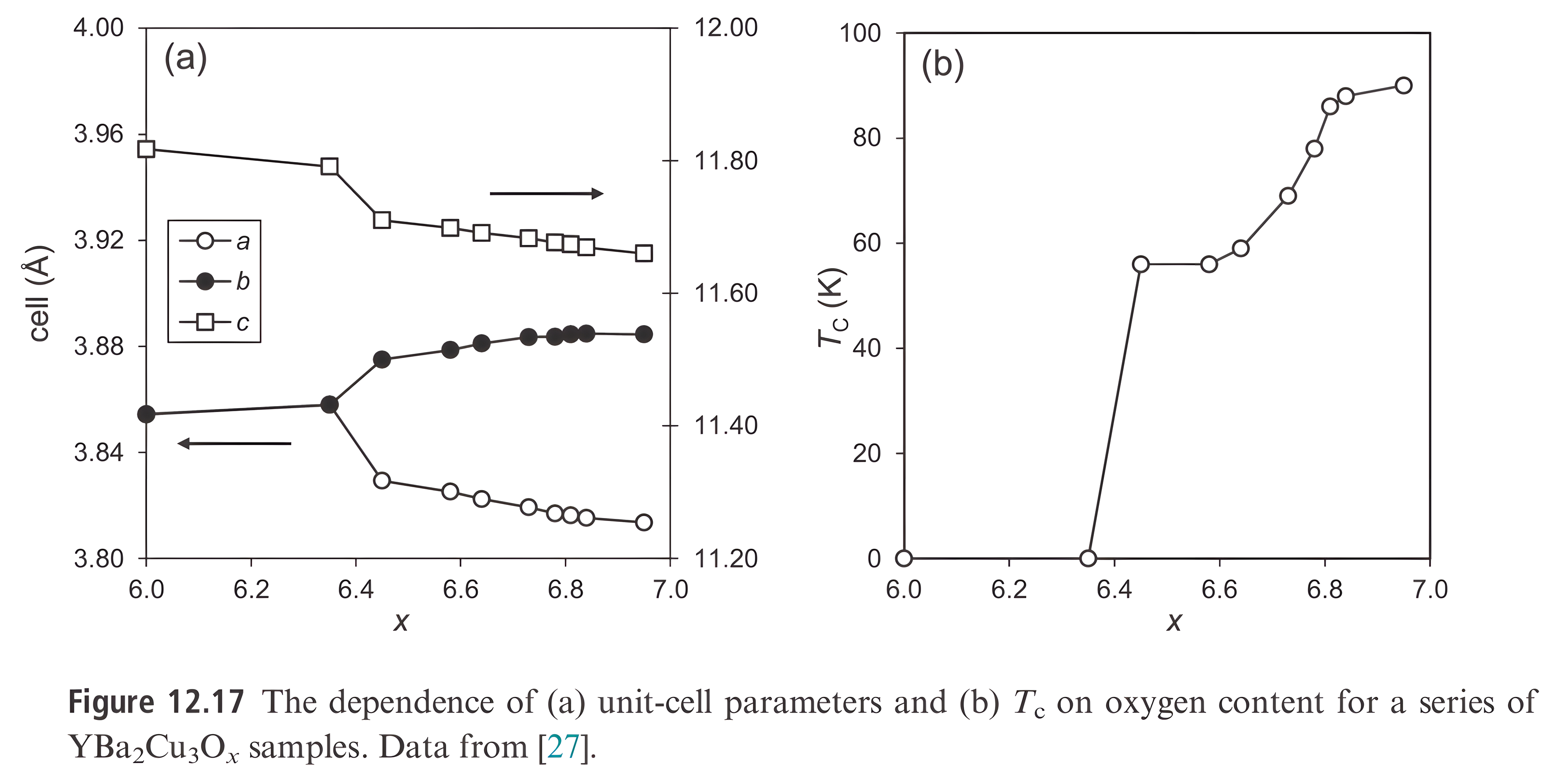
Oxygen Content and $T_c$ in $\mathrm{YBa_2Cu_3O_x}$
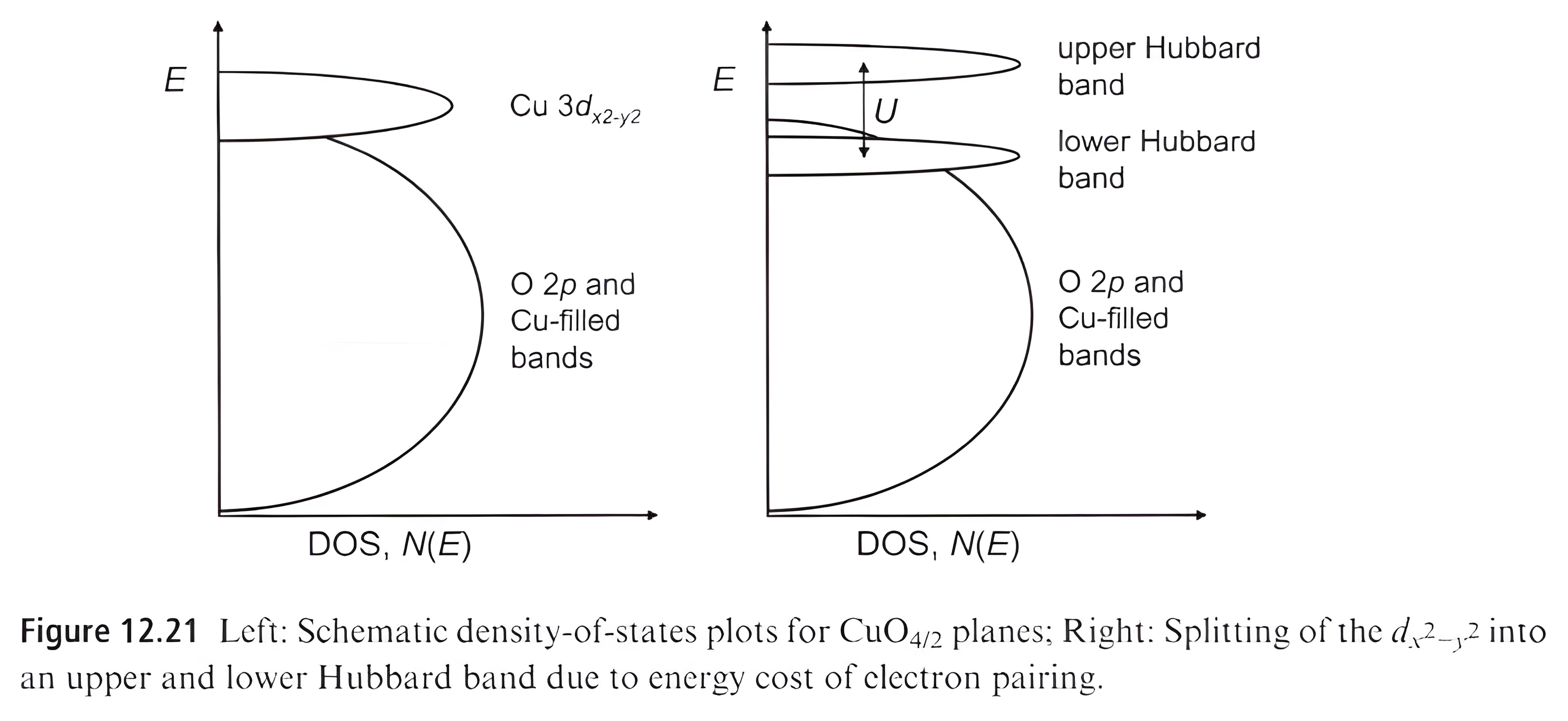
Hubbard Bands and the Mott Insulator
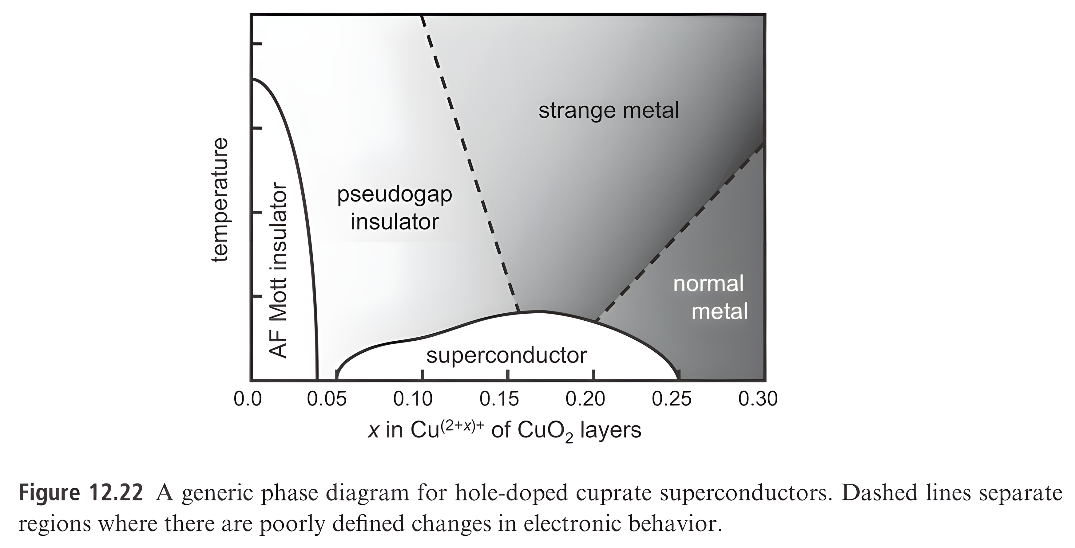
The Cuprate Phase Diagram
Pairing from Electronic Interactions
Pairing seems to come from electronic interactions, not phonons
In ordinary superconductors, electrons attract each other indirectly by distorting the lattice (phonons). In cuprates, that is not strong enough to explain $T_c$ near 100 K.
Instead, the starting point is that the undoped cuprate is an antiferromagnetic Mott insulator: neighboring Cu spins strongly prefer to be opposite. When you dope holes into this system, you
- destroy long-range antiferromagnetic order
- but keep strong, short-range “up–down” tendencies that fluctuate in space and time
These time-dependent local antiferromagnetic patterns are what people mean by spin fluctuations.
They act as a kind of magnetic glue:
- an electron moving through the lattice disturbs the spin background
- another electron can lower its energy by moving in a way that fits this disturbed pattern
- the net effect is an effective attraction between electrons, even though the bare interaction is repulsive
So instead of an ”electron–phonon” attraction, cuprates likely have an ”electron–spin-fluctuation” attraction that binds electrons into Cooper pairs.
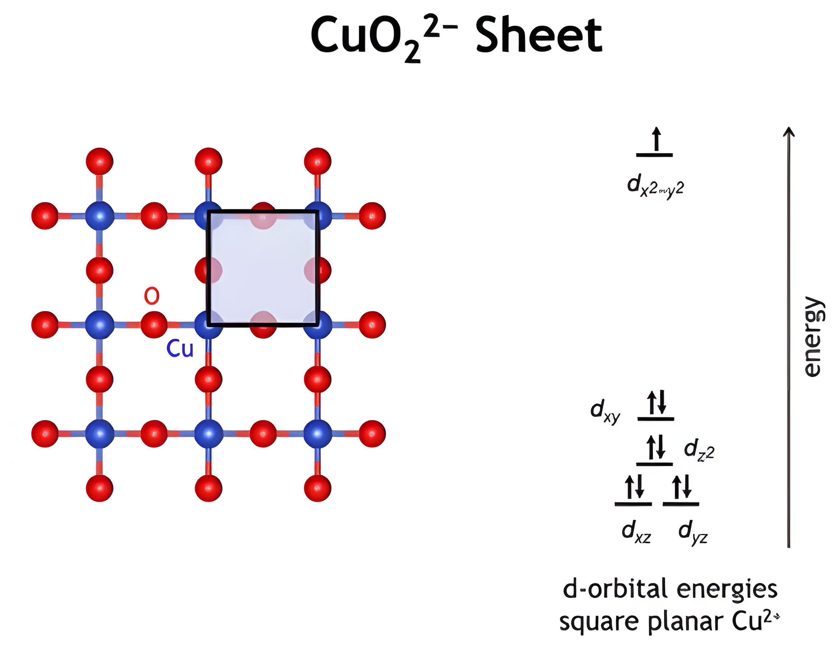
The $\mathrm{CuO_2}$ Sheet
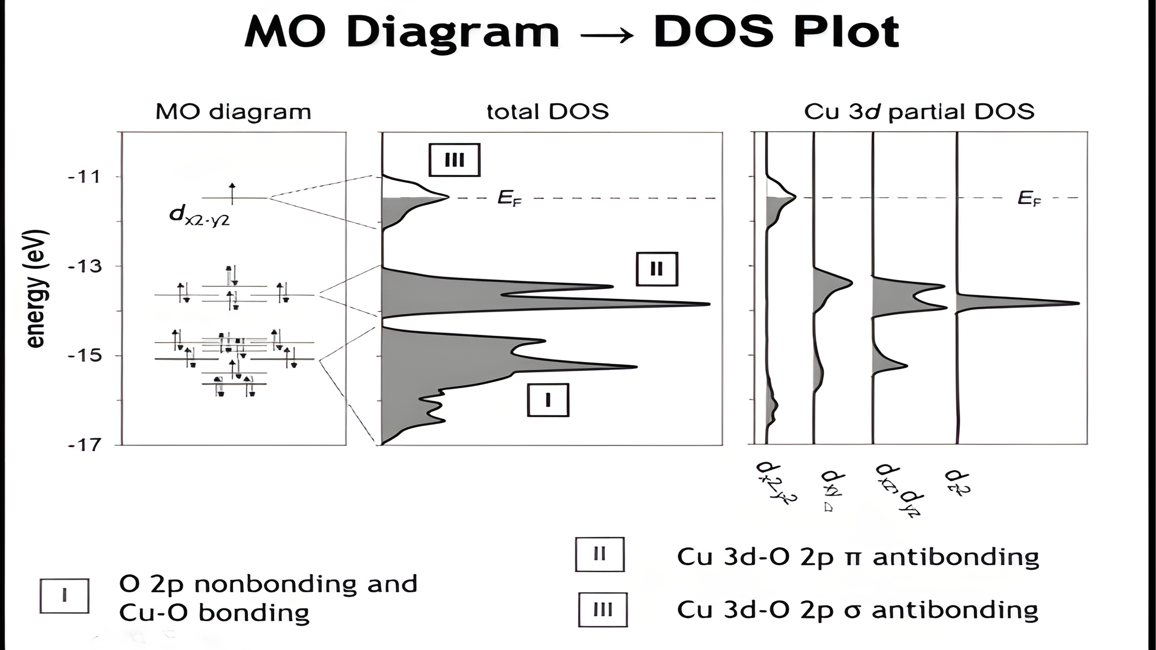
MO Diagram → DOS Plot
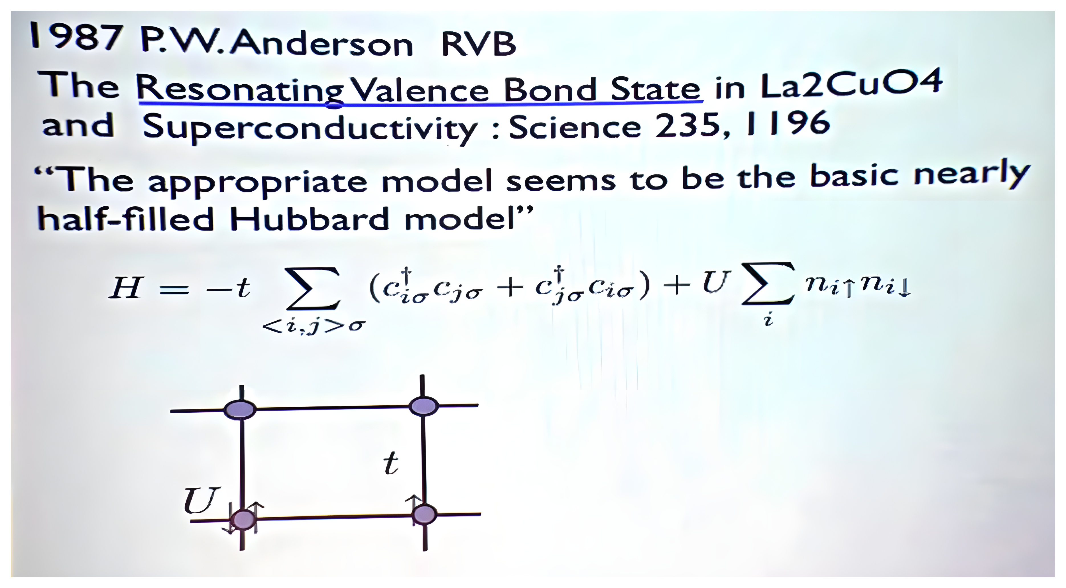
Anderson and the Resonating Valence Bond
Stripes in the Hubbard Model
Coexistence of superconductivity with partially filled stripes in the Hubbard model
Hao Xu†, Chia-Min Chung†, Mingpu Qin, Ulrich Schollwöck, Steven R. White, Shiwei Zhang*
READ THE FULL ARTICLE AT
https://doi.org/10.1126/science.adh7691
Illustration of the ground-state properties of the t-t'-U Hubbard model. Dome-like structures in the superconducting order parameter resemble the $T_c$ domes in the cuprates. With electron doping, superconductivity is accompanied by antiferromagnetic Néel correlations. With hole doping, superconductivity coexists with anti-ferromagnetic correlations that are modulated by a wavelength smaller than 2/doping, with moderate hole-density correlation peaks at the nodes.
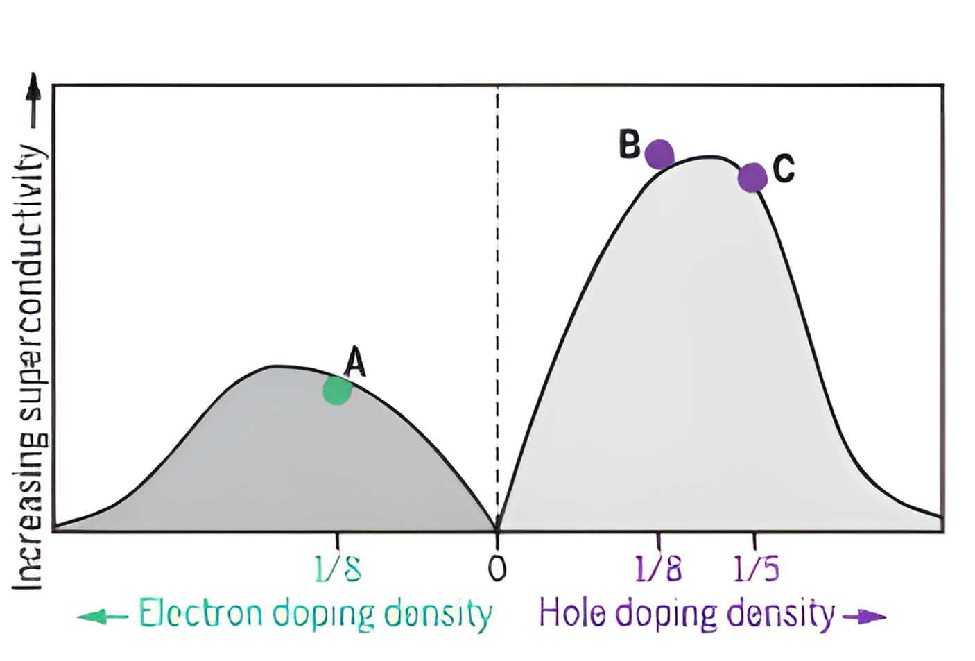
Increasing superconductivity; Electron doping density (1/8, point A); Hole doping density (1/8, point B; 1/5, point C).
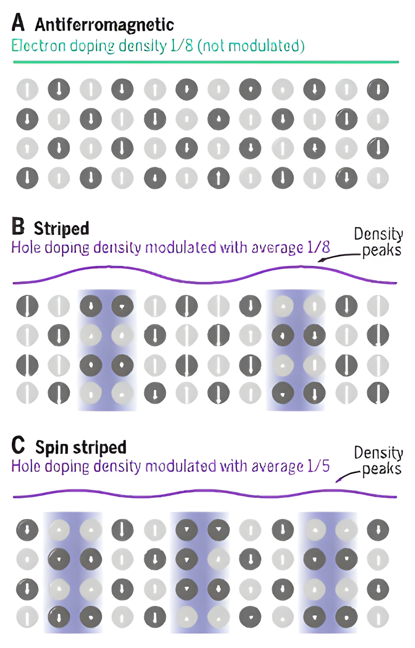
A Antiferromagnetic: Electron doping density 1/8 (not modulated). B Striped: Hole doping density modulated with average 1/8; Density peaks. C Spin striped: Hole doping density modulated with average 1/5; Density peaks.
Electronic Models Reproduce Superconductivity
Simple electronic models now reproduce superconductivity
The Hubbard model is the standard “minimal” model to capture strong electronic correlations on a lattice:
- electrons live on a square lattice (like Cu sites)
- they can hop to neighboring sites with amplitude t
- if two electrons land on the same site, they pay a large energy penalty U (strong on-site repulsion)
At half-filling (one electron per site), and for large U, the Hubbard model naturally gives a Mott insulating antiferromagnet, just like undoped cuprates.
Practice questions
Work the Lecture 21 practice questions before the next class. They cover zero resistance and the Meissner effect, type I and type II behaviour, the magnetic response quantities and susceptibility, the thermodynamic signature at $T_c$, Cooper pairing and the BCS gap, and the cuprates from YBa₂Cu₃O₇ to the Hubbard-model picture of the pairing glue.
Open the Lecture 21 practice questions
Every question carries a worked explanation, so you can check your reasoning as you go.