CHEM 548: Materials Chemistry

Lecture 19: Electrical Conductivity: the Drude and Free Electron Models

Mon 11/09/2026 · Meeting 21

Reading: Woodward, Karen, Evans, and Vogt, Solid State Materials Chemistry
Ch. 10 §10.2

Learning Objectives: The Drude Model

Electrical Conductivity and the Drude Model

  • Distinguish between extrinsic (I, V, R) and intrinsic (J, E, σ, ρ) electrical properties
  • Apply the Drude model to describe electron behavior as an ideal gas in metals
  • Calculate key parameters: drift velocity, electron mobility, mean free path, and relaxation time
  • Derive the relationship between conductivity, carrier concentration, and mobility (σ = neμ)
  • Estimate conductivity parameters for simple metals using the Drude model
  • Recognize the limitations and failures of the Drude model in predicting temperature dependence and trends across different metals

Electrical Properties of Materials | Materials Science & Chemistry

Ohm's Law
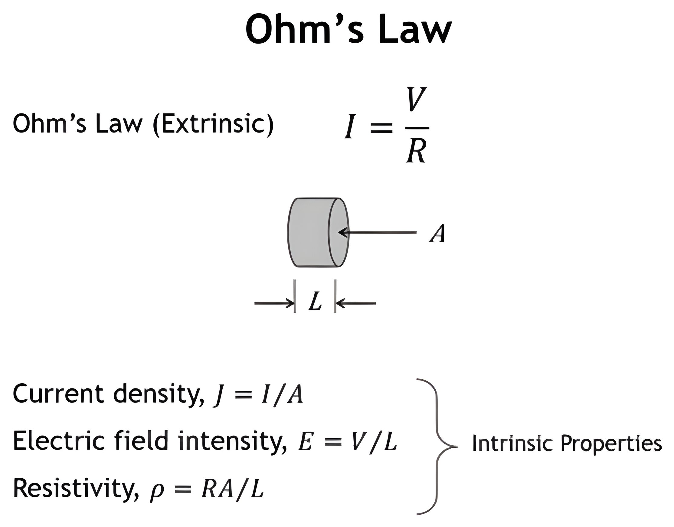
Ohm's law I equals V over R beside a cylindrical sample with cross-sectional area A and length L, and the intrinsic properties: current density J equals I over A, electric field intensity E equals V over L, and resistivity rho equals R A over L.

From Ohm's Law to Conductivity

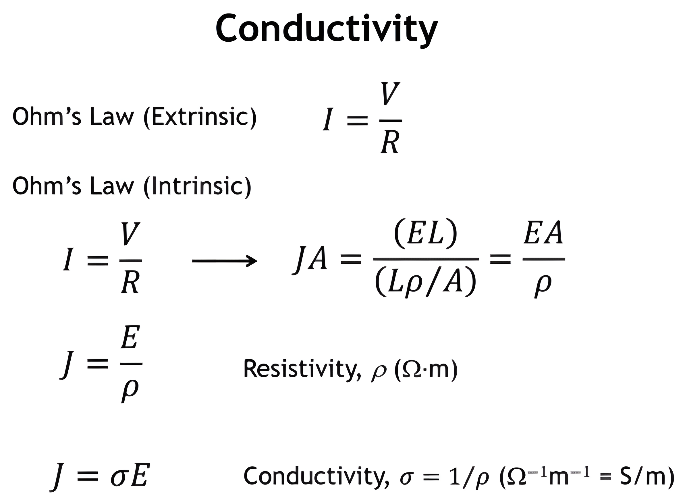
Recasting Ohm's law into intrinsic form: J A equals E L over L rho over A, which reduces to J equals E over rho, and J equals sigma E with conductivity sigma equal to one over rho.

Conductivity of Materials

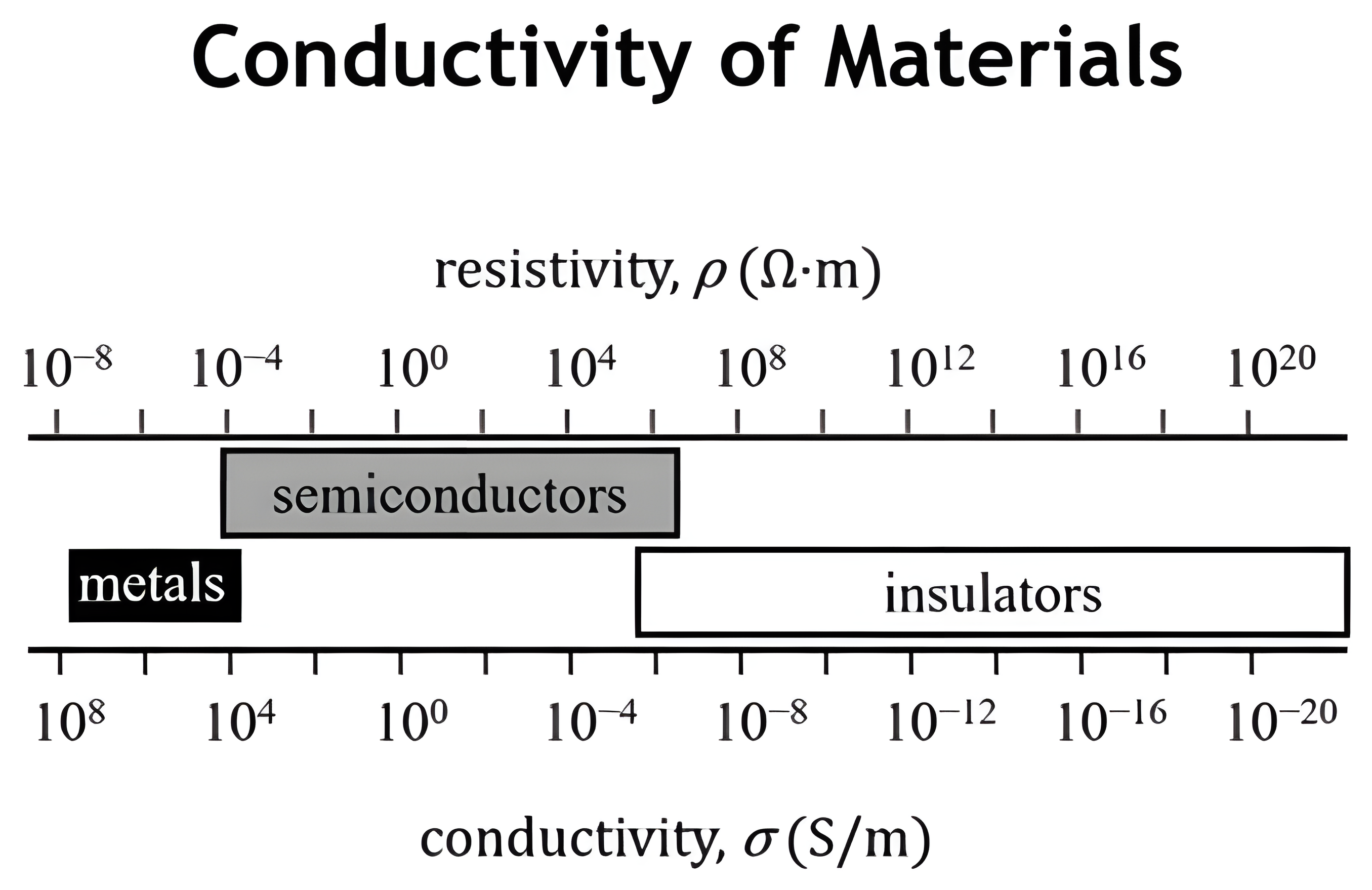
Logarithmic scales of resistivity and conductivity spanning 28 orders of magnitude, with metals at high conductivity, semiconductors in the middle, and insulators at low conductivity.

Conductivity of Select Materials

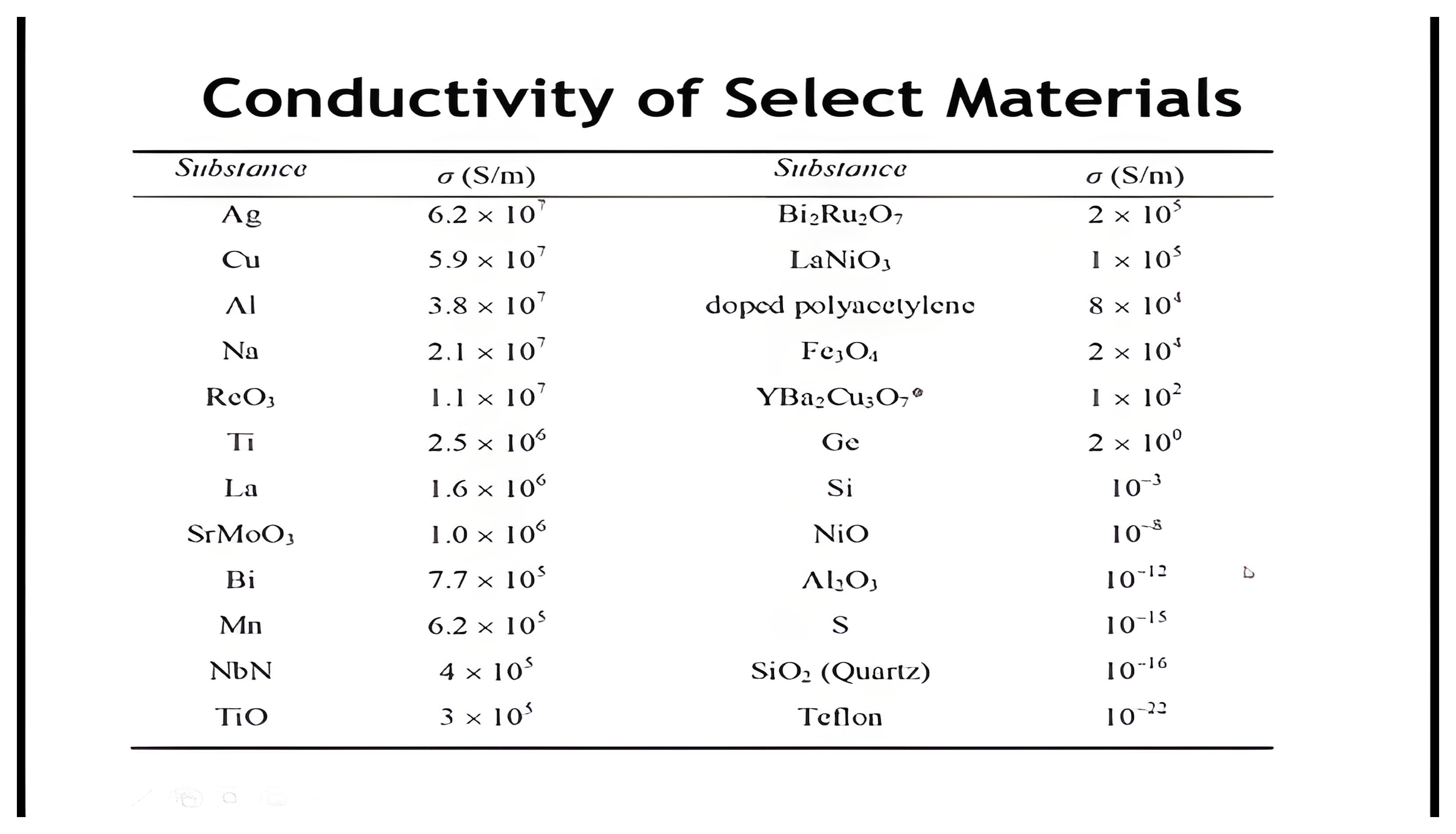
Table of conductivities in siemens per meter for selected materials, from silver, copper, and aluminum near ten to the seventh down through oxides and semiconductors to quartz and Teflon near ten to the minus sixteen and below.

The Drude Model: a Free Electron Gas

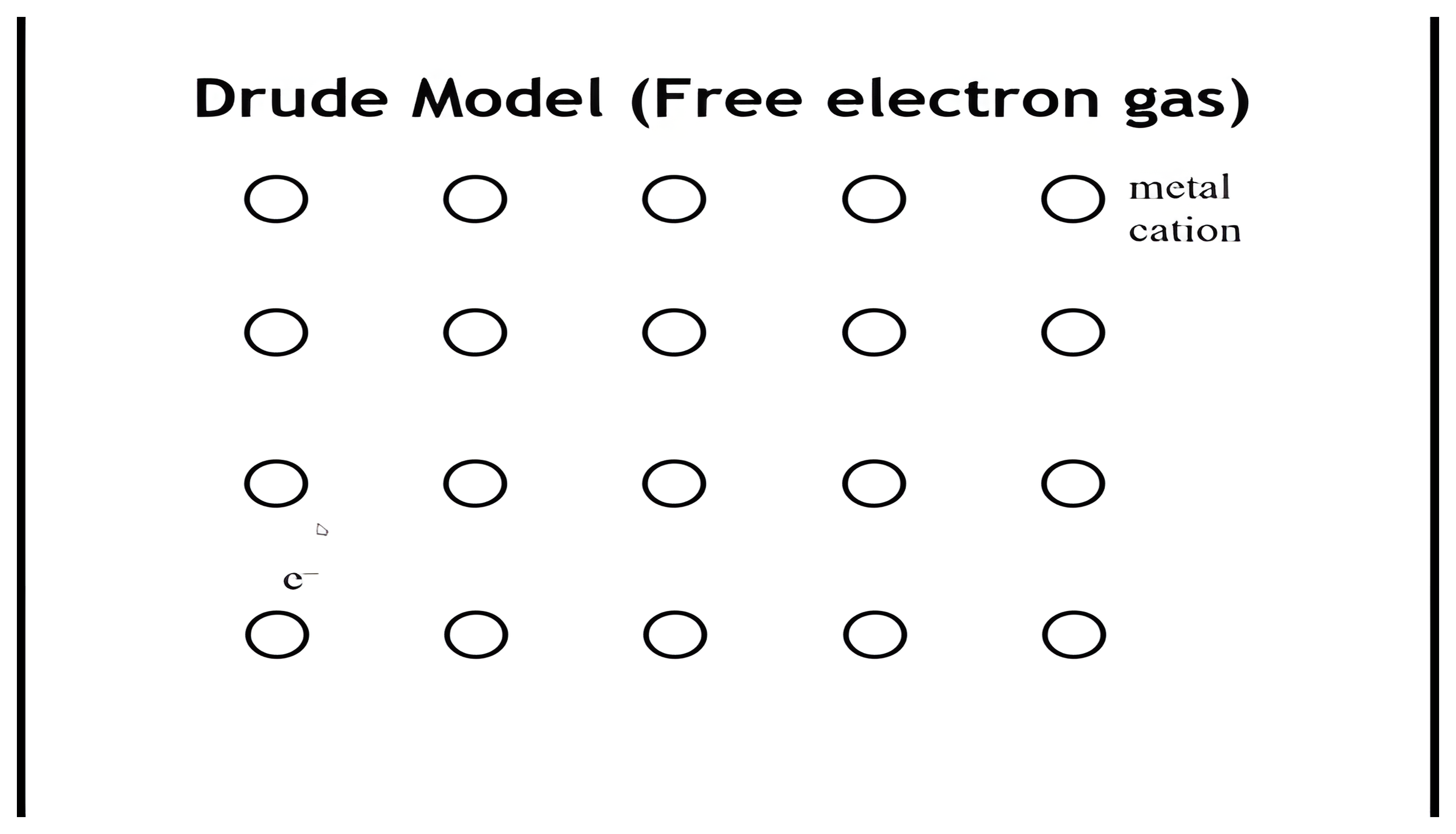
A grid of metal cations with an electron label; a click traces the electron's zigzag path as it collides with ions in the lattice and redirects at each collision.

The Boltzmann Distribution

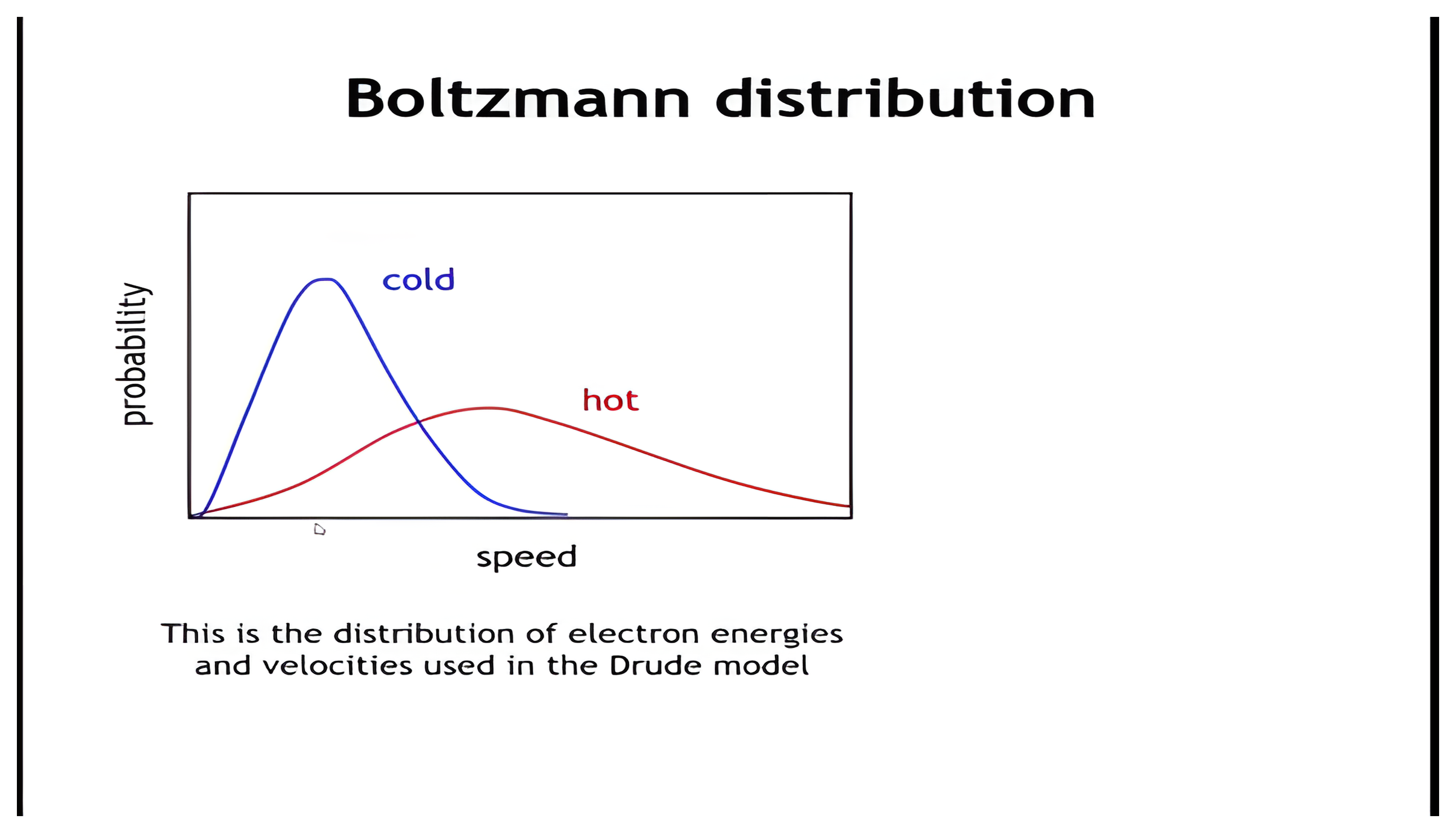
Boltzmann probability distributions of electron speed for a cold gas peaked at low speed and a hot gas spread to higher speeds; a click adds the average energy three halves k T and the root-mean-square velocity formula giving about ten to the fifth meters per second at 300 kelvin.

Mean Free Path and Relaxation Time

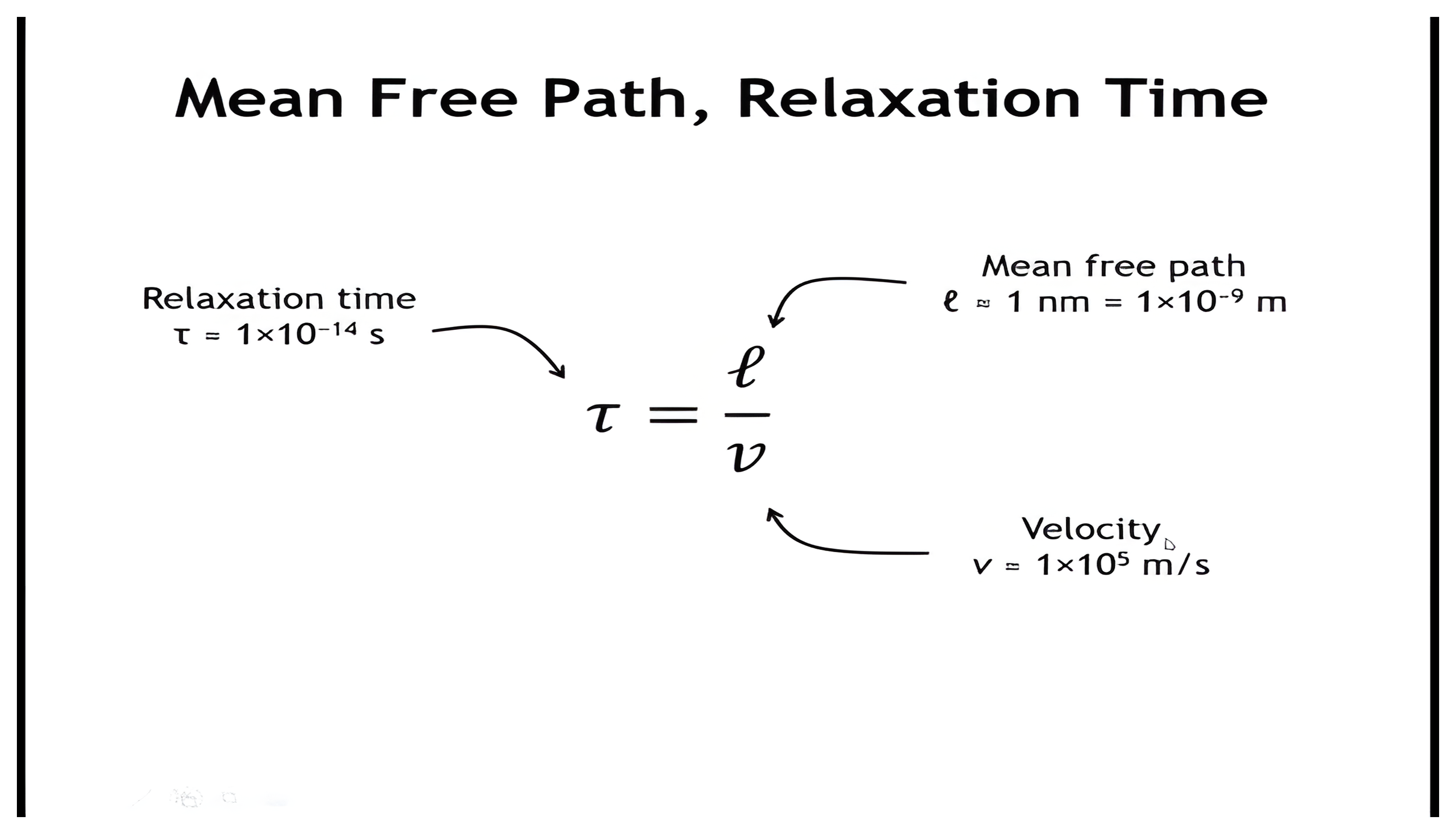
The relaxation time tau equals mean free path over velocity, annotated with mean free path approximately one nanometer, velocity ten to the fifth meters per second, and relaxation time approximately ten to the minus fourteen seconds.

Drift Velocity

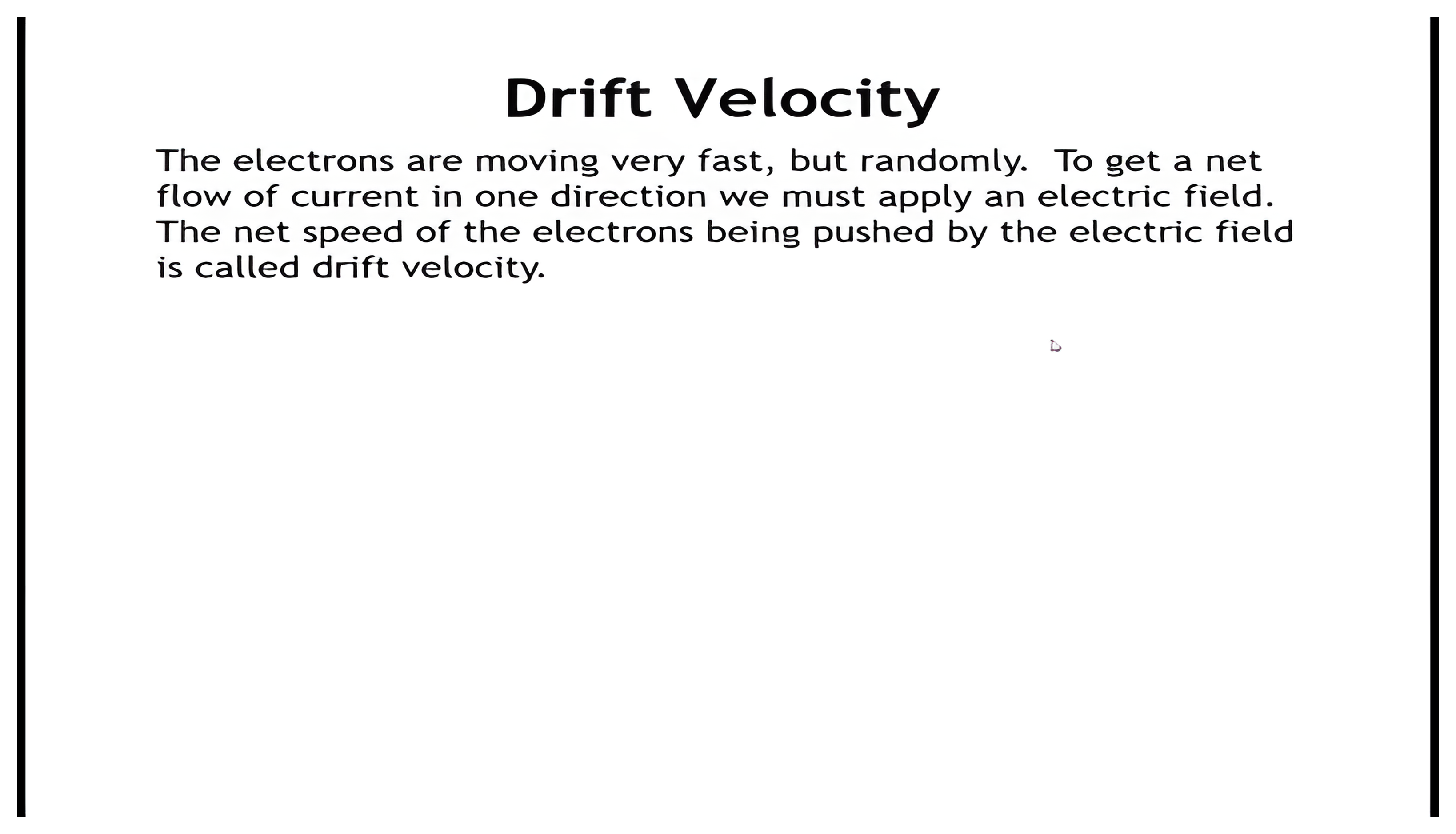
Definition of drift velocity as the net speed of electrons pushed by an electric field; clicks add Newton's law F equals m a, the force e E equals m e a, the acceleration, the drift velocity v d equals a tau, and the note that drift velocity is about 0.2 meters per second.

Electron Mobility

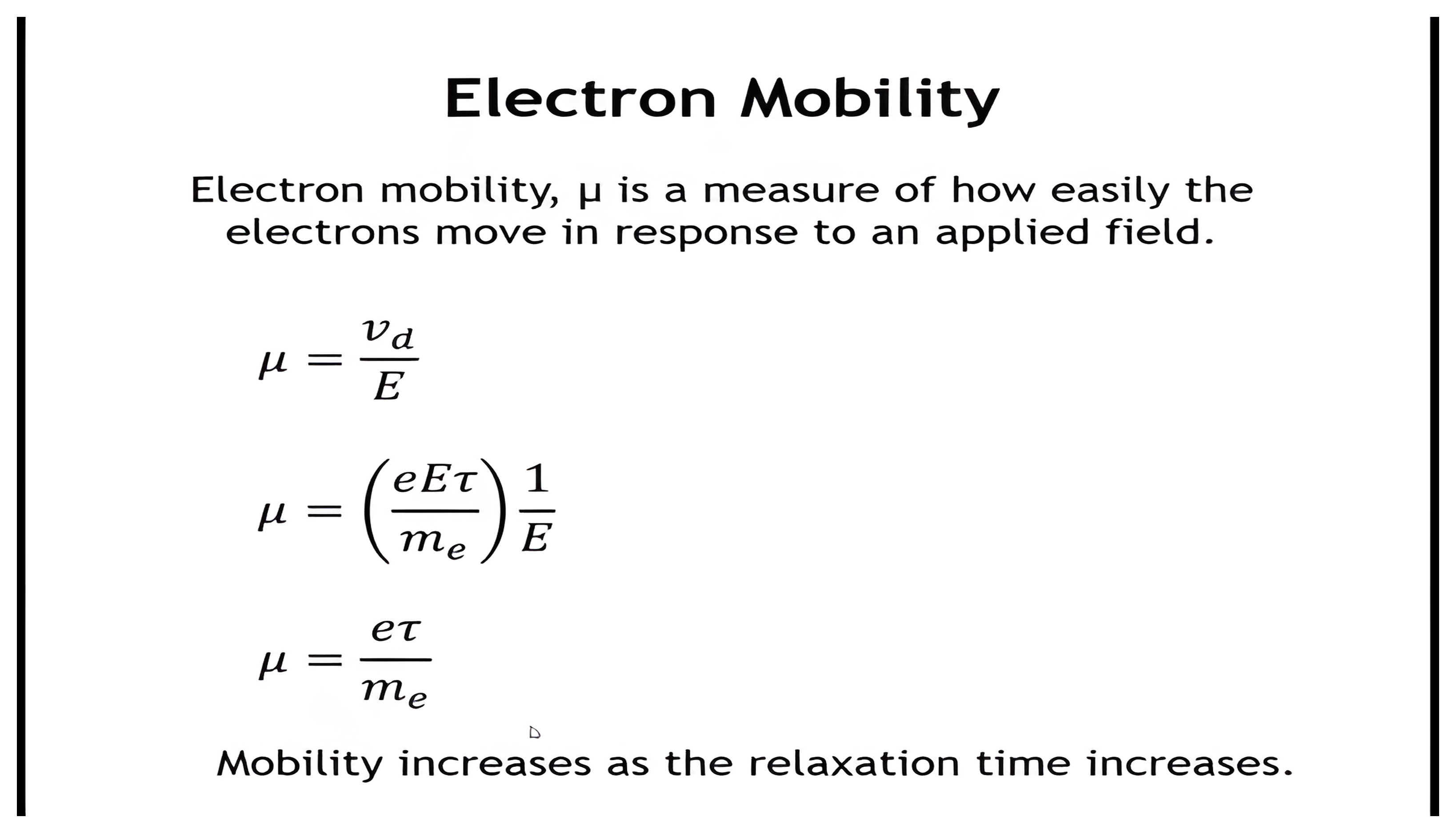
Electron mobility mu defined as drift velocity over electric field, reduced through the drift-velocity expression to mu equals e tau over m e; mobility increases as the relaxation time increases.

Conductivity: $\sigma = ne\mu$

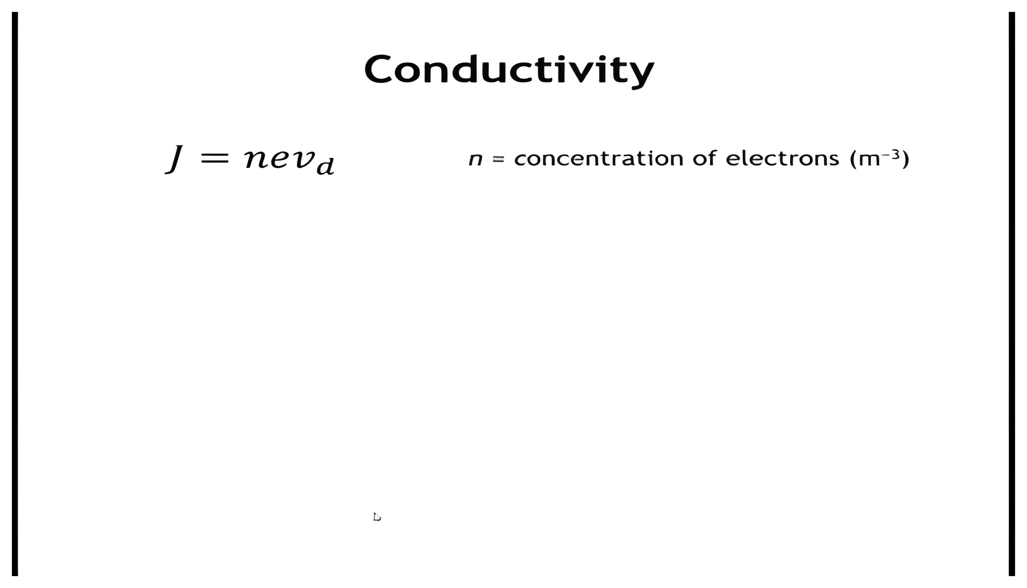
Current density J equals n e v d with n the concentration of electrons; a click substitutes the mobility to give J equals n e mu E, compares with J equals sigma E, and identifies sigma equals n e mu.

Adding Up the Numbers: Sodium

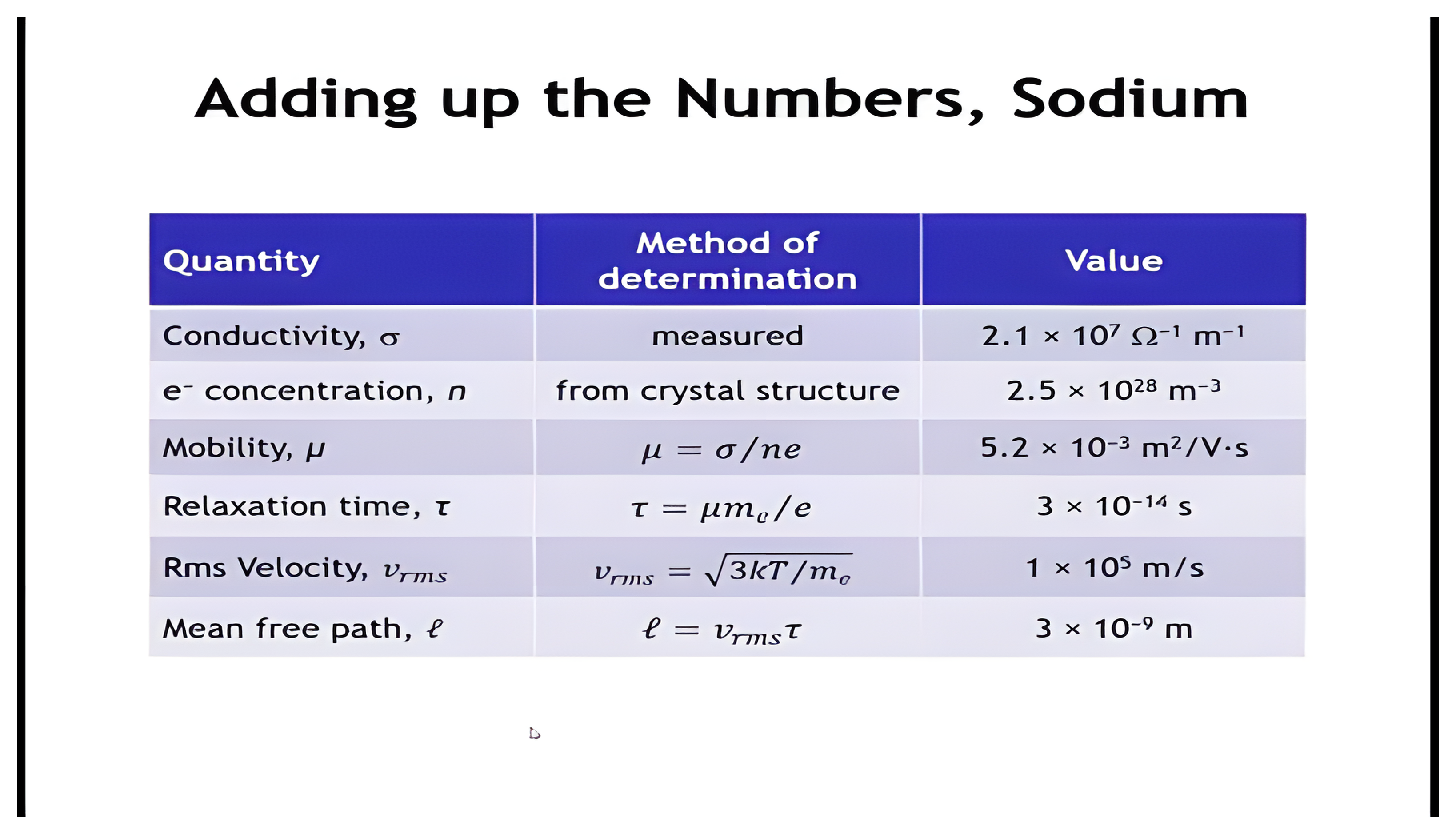
Table of Drude-model quantities for sodium: measured conductivity 2.1 times ten to the seventh, electron concentration 2.5 times ten to the twenty-eighth per cubic meter, mobility 5.2 times ten to the minus third, relaxation time 3 times ten to the minus fourteenth seconds, rms velocity ten to the fifth meters per second, and mean free path 3 nanometers.

Valence Electron Concentration and Conductivity

Table 10.2 Conductivity σ does not scale with the valence-electron concentration n.

Metaln (m⁻³)σ (S/m)Metaln (m⁻³)σ (S/m)
Rb1.1×10²⁸0.8×10⁷Aga5.9×10²⁸6.2×10⁷
K1.3×10²⁸1.4×10⁷Aua5.9×10²⁸4.5×10⁷
Na2.5×10²⁸2.1×10⁷Cua8.4×10²⁸5.9×10⁷
Ca4.6×10²⁸2.9×10⁷Zna13.1×10²⁸1.7×10⁷
Mg8.6×10²⁸2.3×10⁷Sc12.0×10²⁸0.18×10⁷
Al18.0×10²⁸3.8×10⁷Ti20.5×10²⁸0.25×10⁷

a The d subshells of Cu, Ag, Au, and Zn are assumed to be full and are not counted in the valence-electron count.

Why doesn’t σ scale with valence electron concentration, n, once we move beyond the alkali metals?

Check Your Understanding: Which Velocity Carries the Current?
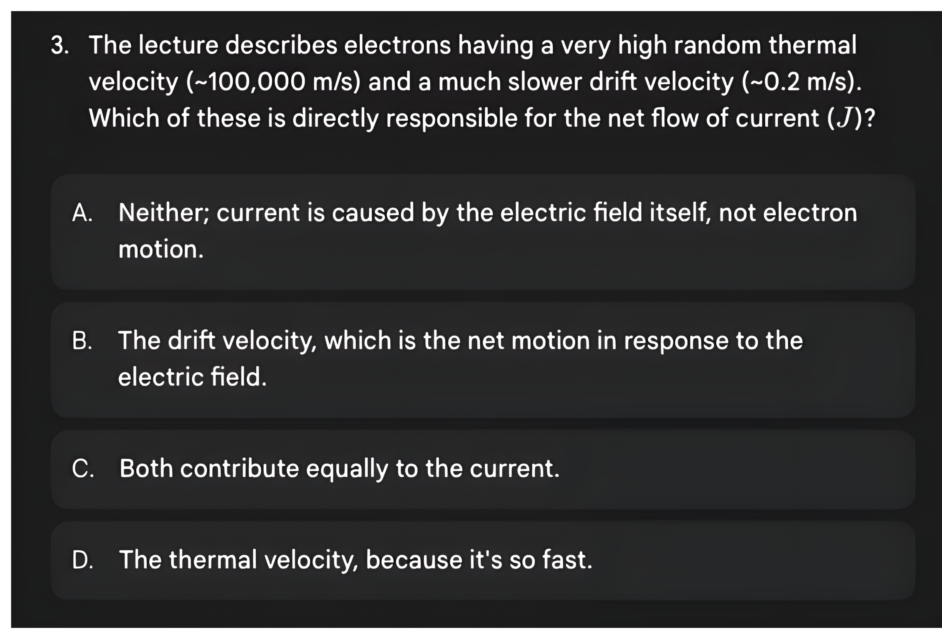
Question 3 asking whether the high random thermal velocity or the much slower drift velocity is directly responsible for the net flow of current, then its answer: the drift velocity, the net motion in response to the electric field.

Learning Objectives: Quantum Mechanics and Metallic Conductivity

Quantum Mechanics and Metallic Conductivity

  • Explain the transition from the Drude model to the free electron model and identify the key quantum mechanical principles incorporated in the free electron model
  • Describe the parabolic E(k) relationship in the free electron model and relate it to the particle-in-a-box treatment
  • Connect effective mass (m*) to band curvature and predict how band structure affects carrier mobility and conductivity
  • Apply the Fermi-Dirac distribution to explain which electrons contribute to electrical conductivity and why only states near the Fermi level matter
  • Explain the temperature dependence of metallic conductivity, including the role of phonon scattering and residual resistivity
  • Predict relative conductivities across the periodic table by analyzing band structure, particularly distinguishing between d-band and s-band contributions to transport
  • Justify why coinage metals (Cu, Ag, Au) exhibit exceptionally high conductivities compared to transition metals based on their electronic band structures

The Potential in the Free Electron Model
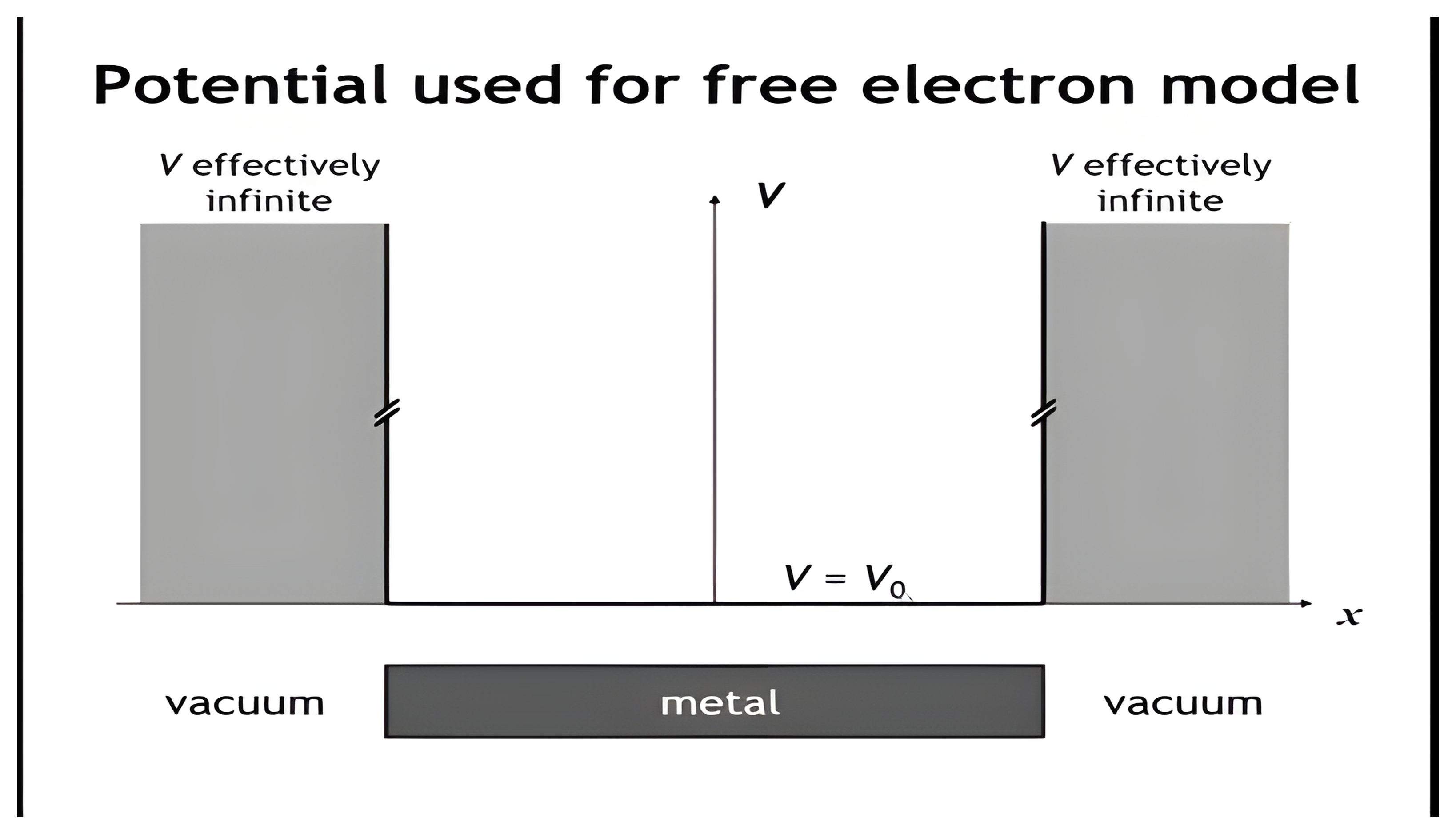
The potential used for the free electron model: V equals V zero inside the metal and effectively infinite in the vacuum on either side, trapping the electrons inside the crystal like a particle in a box.

The Free Electron Model

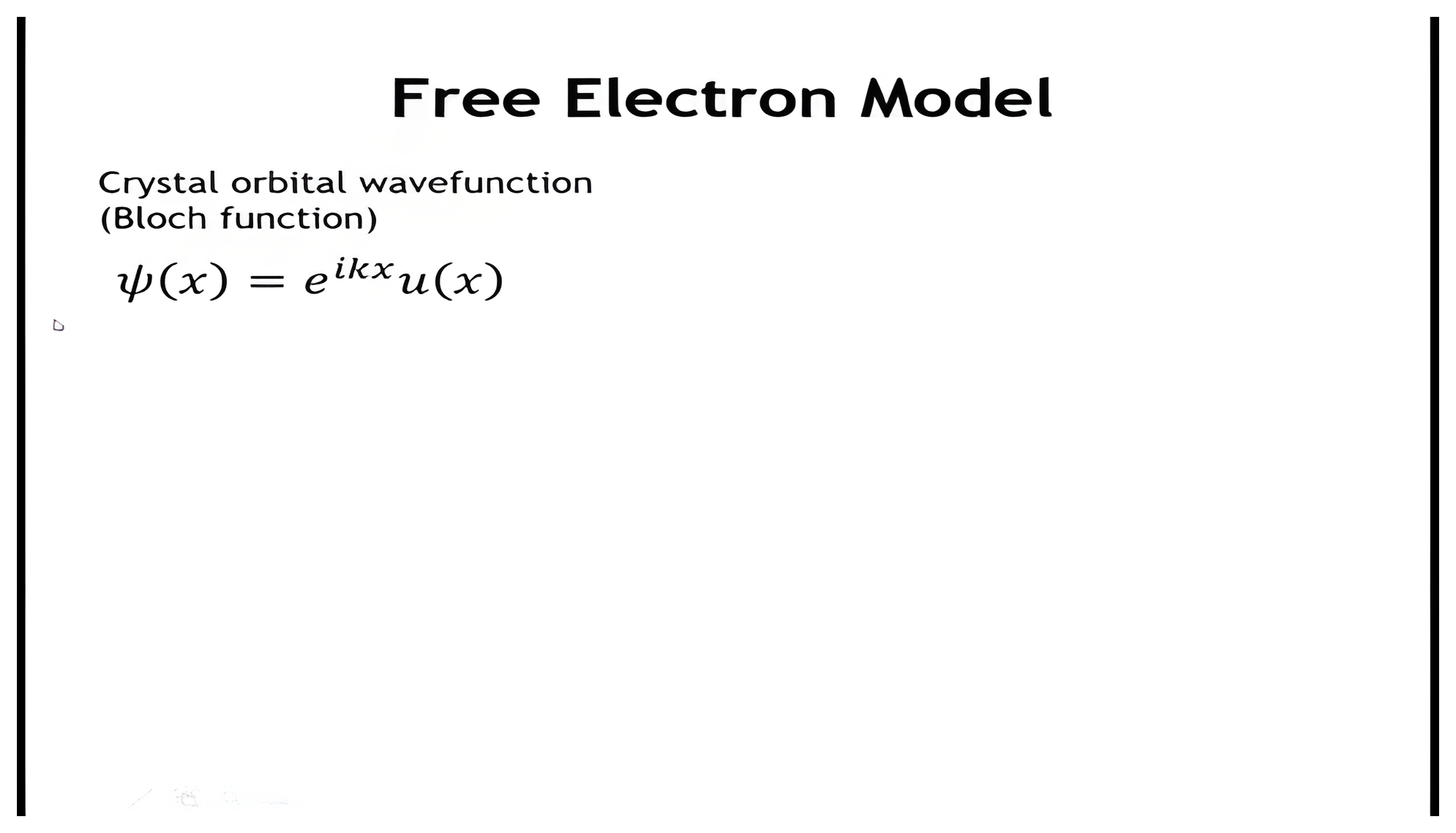
The Bloch function psi of x equals e to the i k x times u of x; clicks set u of x to one, apply the time-independent Schroedinger equation to give E equals V zero plus h-bar squared over two m e times k squared, and draw the particle-in-a-box wave functions oscillating faster as k increases.

The Free Electron Band Structure

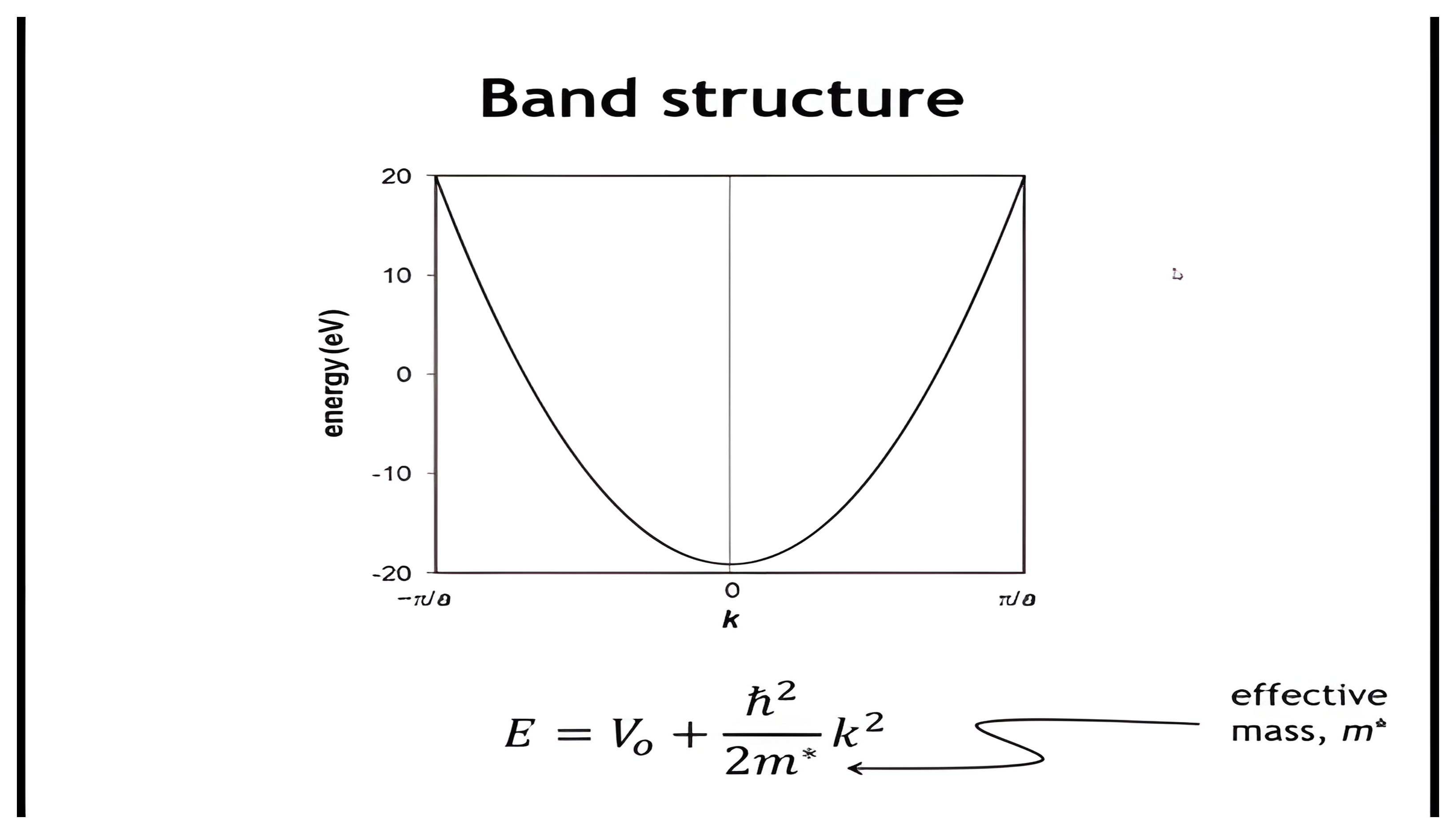
The free electron band structure: a parabola of energy versus k from minus pi over a to pi over a, following E equals V zero plus h-bar squared over two m-star times k squared, with the effective mass m-star labeled.

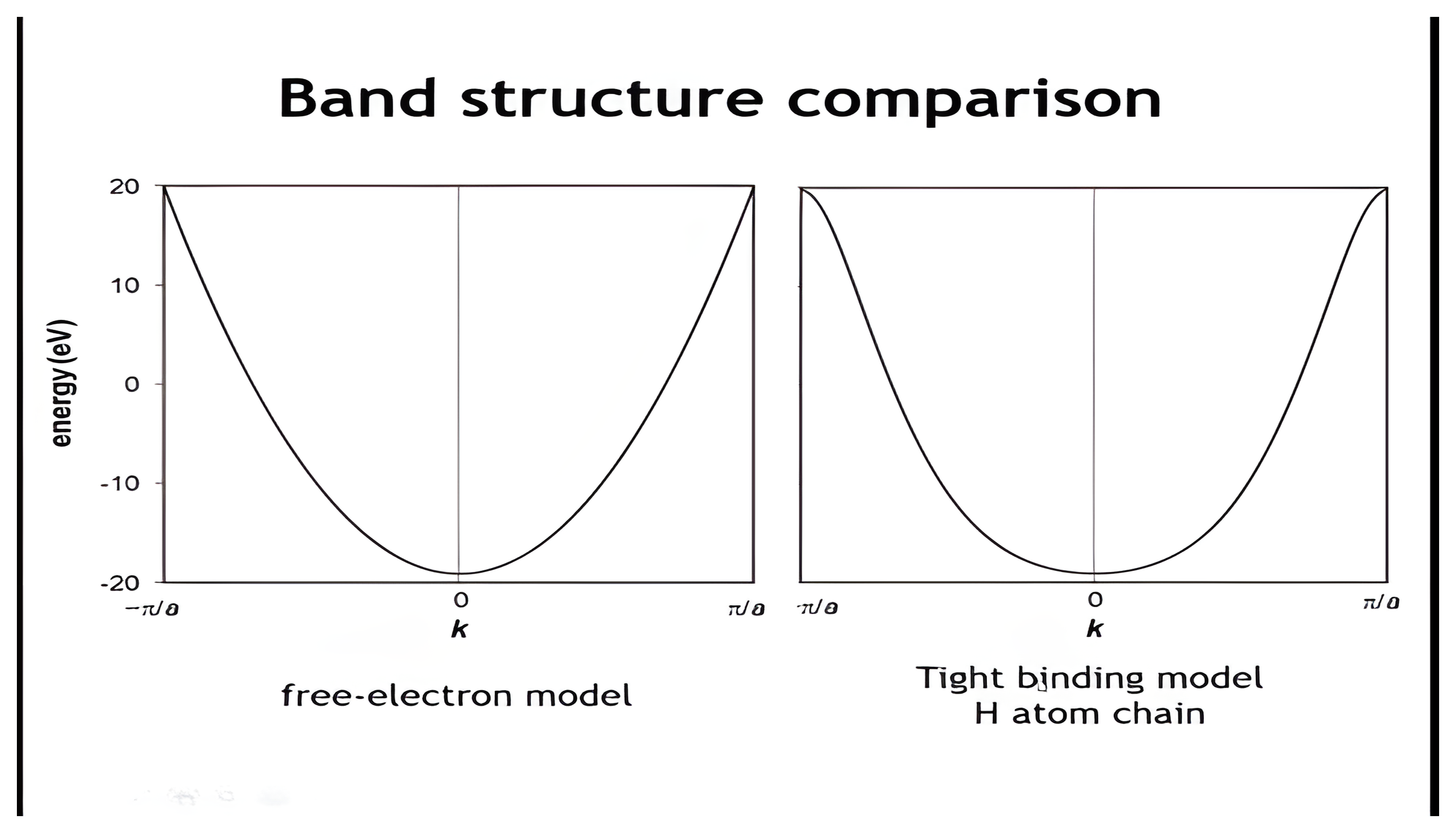
Band Structure Comparison

Side-by-side band structures: the purely parabolic free-electron model and the tight binding model for a hydrogen atom chain, which flattens near the zone edges.

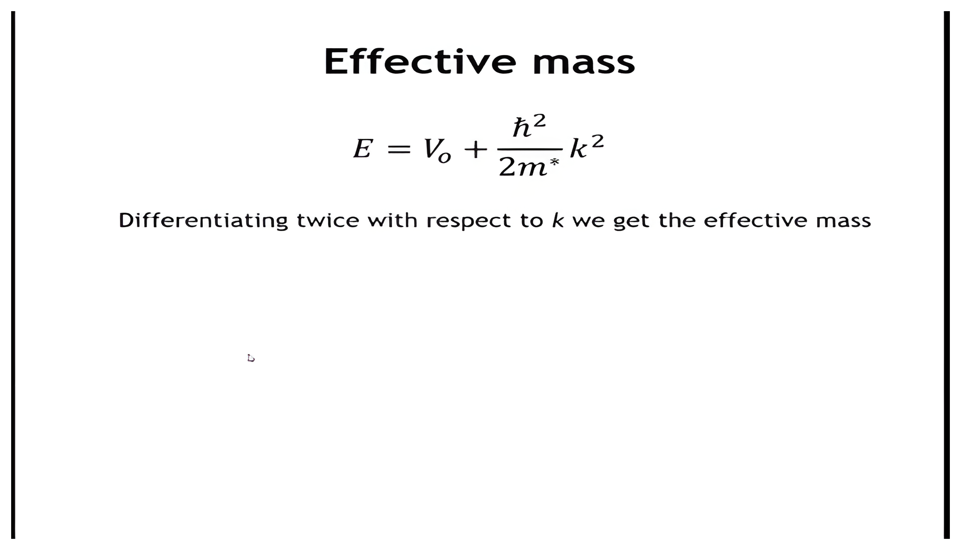
Effective Mass

The energy expression E equals V zero plus h-bar squared over two m-star times k squared; clicks add the second derivative giving m-star equals h-bar squared over the second derivative of E with respect to k, a red circle highlighting the energy expression with the takeaway that wide bands mean large curvature and small effective mass, remove the circle, and add the mobility relation mu equals e tau over m-star.

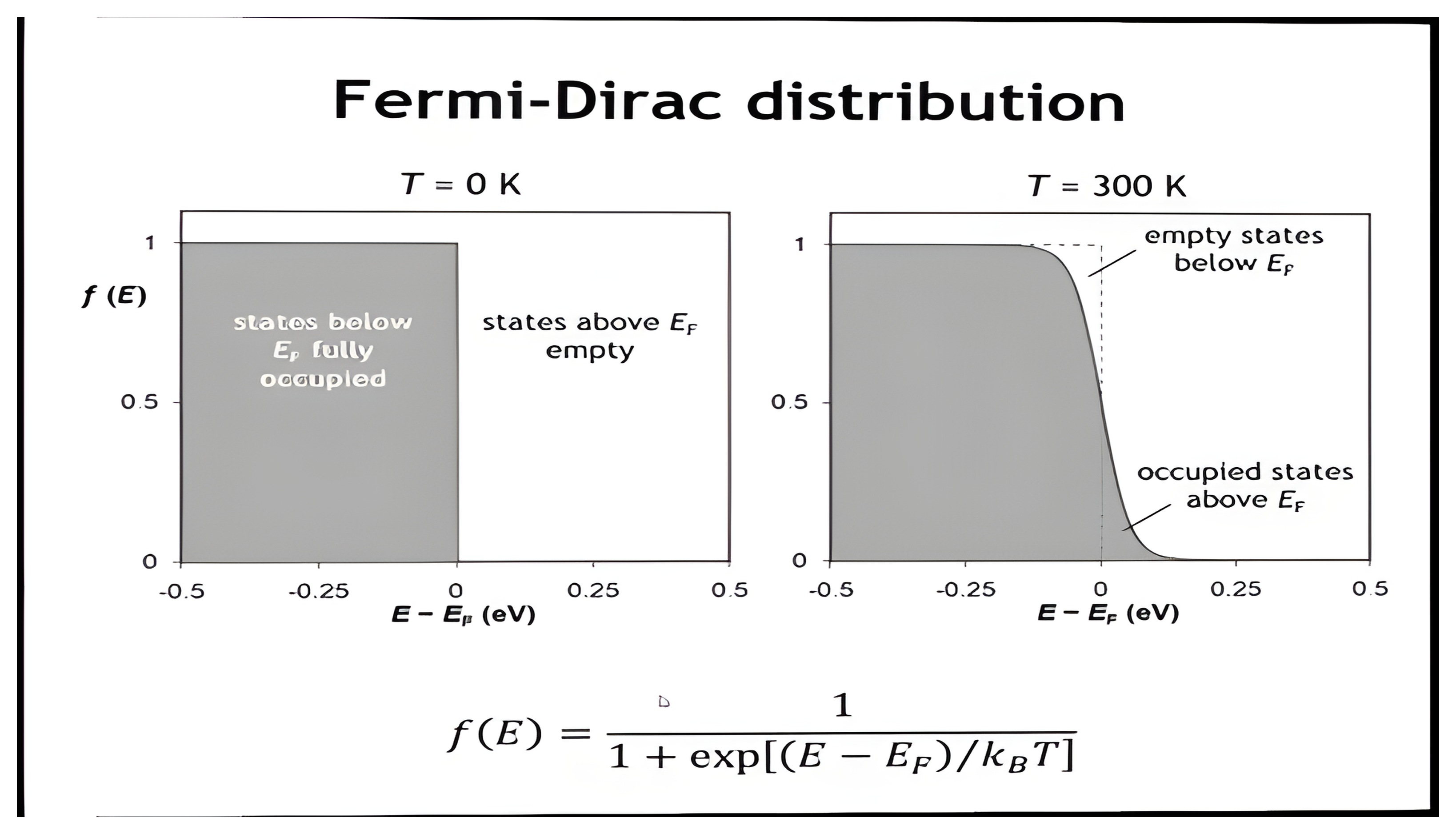
The Fermi-Dirac Distribution

The Fermi-Dirac distribution at zero kelvin, a sharp step with states below the Fermi energy fully occupied, and at 300 kelvin, where the step smears so some states above the Fermi energy are occupied and some below are empty; the function f of E equals one over one plus the exponential of E minus E F over k B T.

Density of States in the Free Electron Model
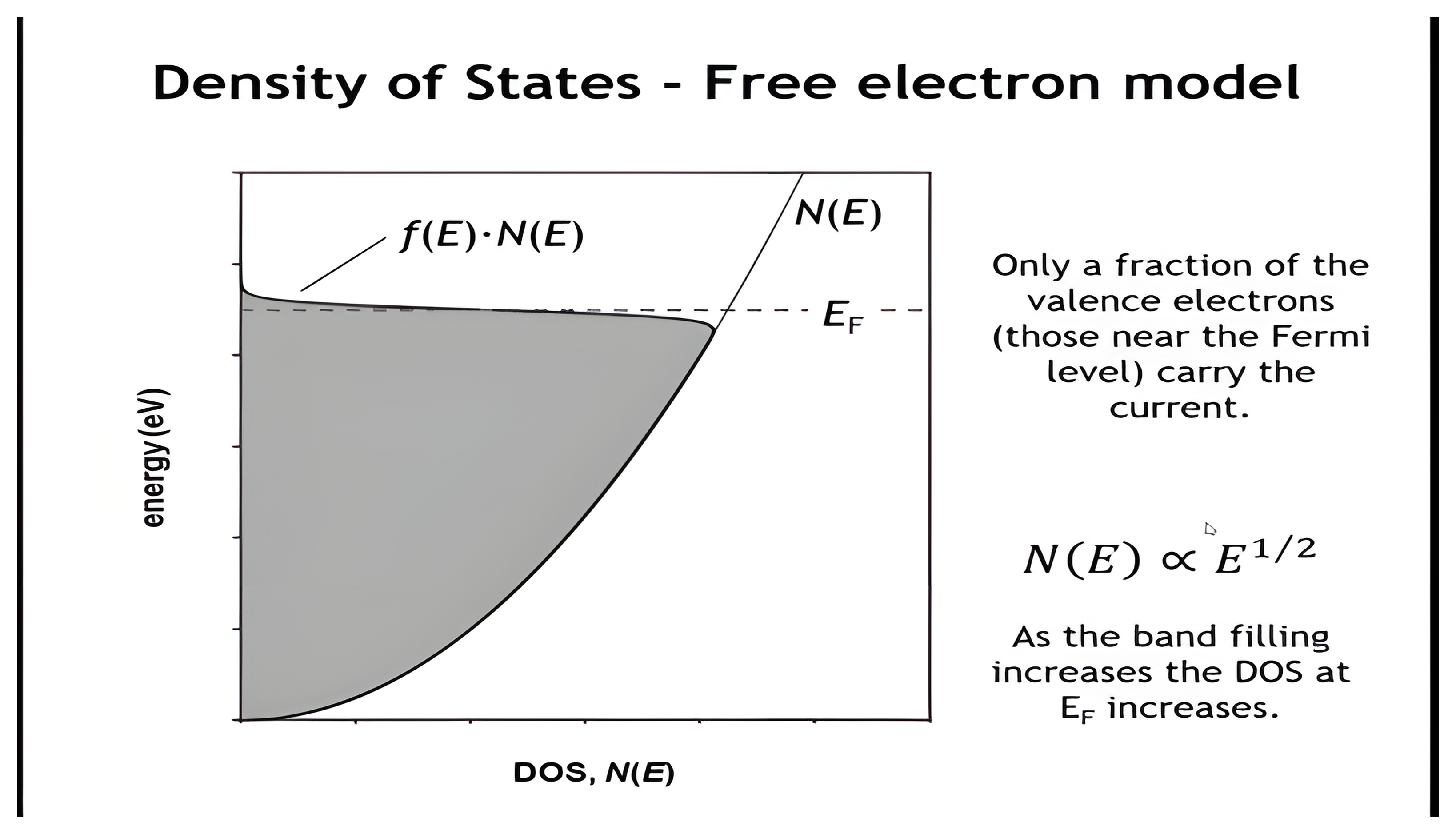
The free-electron density of states rising as the square root of energy, with the occupied states f of E times N of E shaded up to the Fermi energy; only the fraction of valence electrons near the Fermi level carries the current.

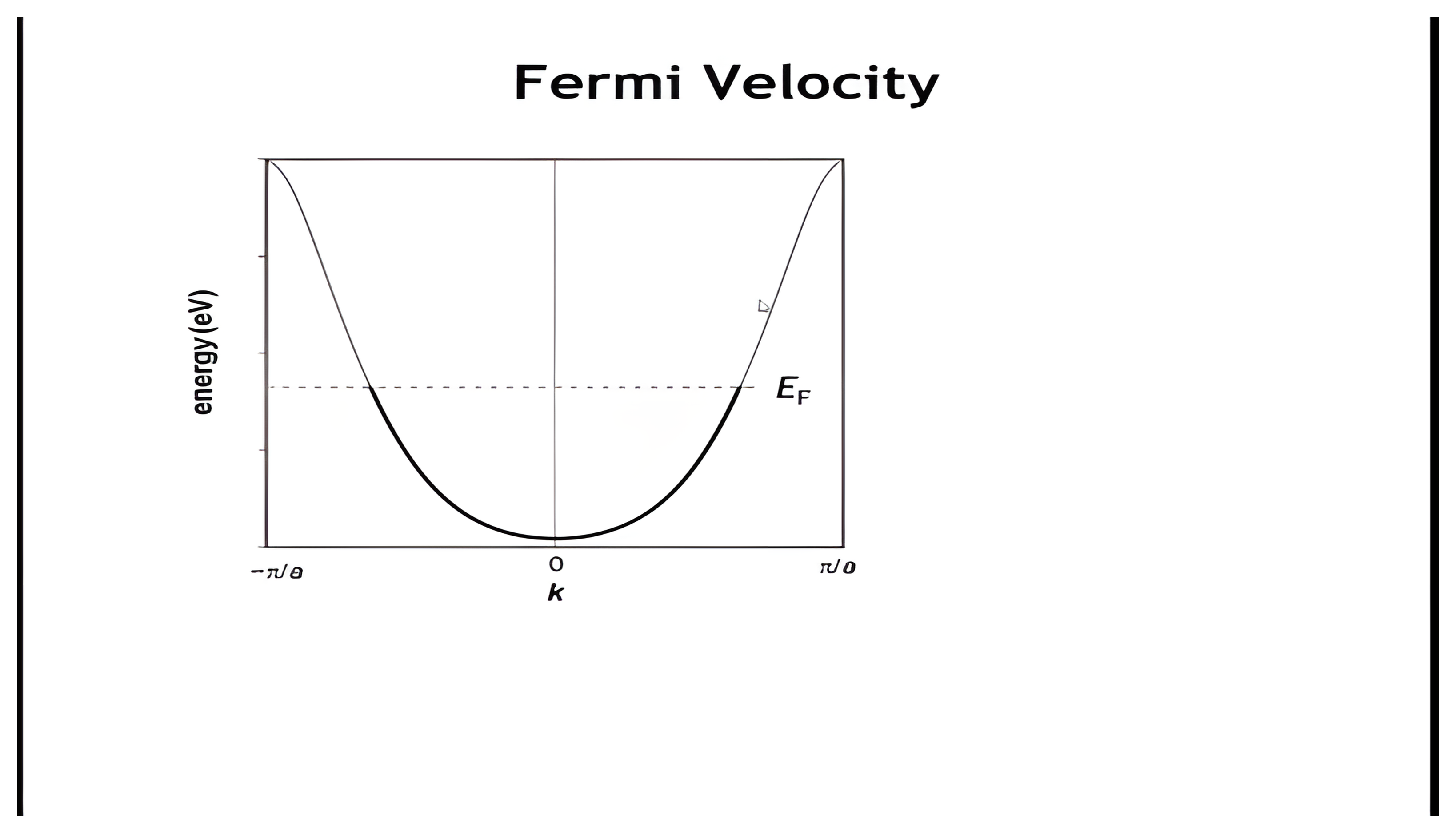
Fermi Velocity

The filled free-electron parabola up to the Fermi energy; clicks add the momentum relations p equals h-bar k, m-star v equals h-bar k, and v equals h-bar k over m-star, then the Fermi velocity v F equals the square root of two E F over m-star.

Uncompensated Electrons Carry the Current
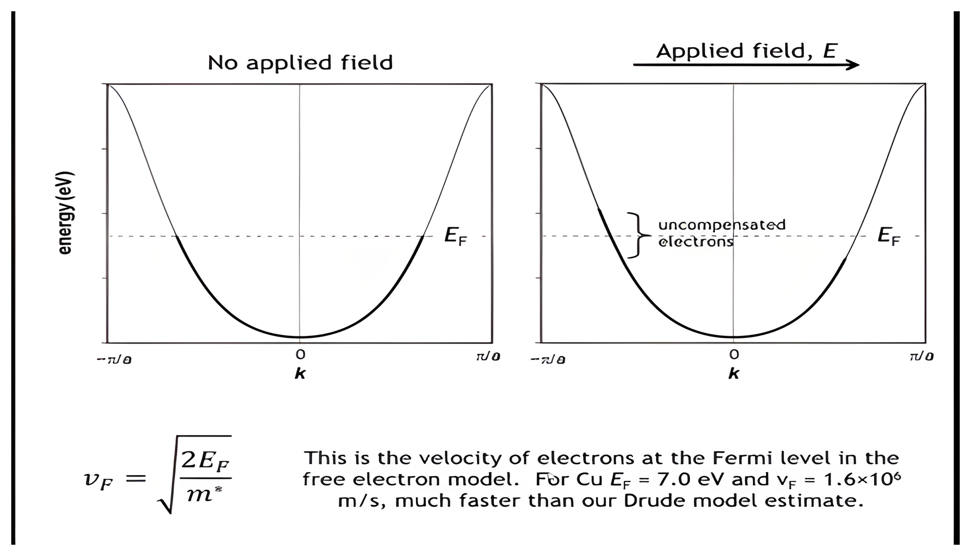
Filled free-electron parabolas with no applied field and with an applied field, where the electron distribution shifts in k and a bracket marks the uncompensated electrons near the Fermi energy; for copper the Fermi energy is 7.0 electron volts and the Fermi velocity 1.6 times ten to the sixth meters per second.

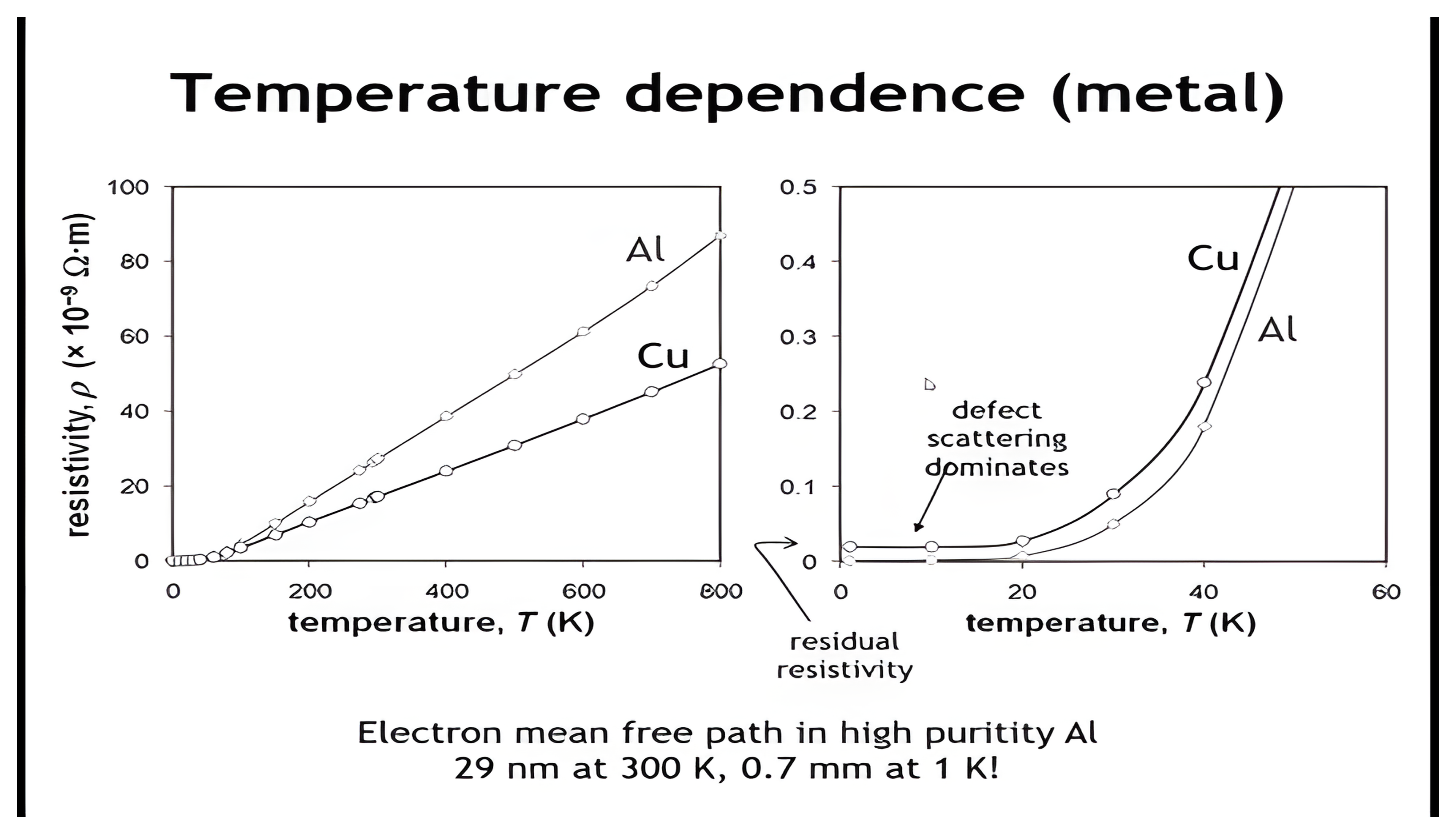
Temperature Dependence of Metals

Resistivity of aluminum and copper versus temperature: linear decrease on cooling from 800 kelvin, then a plateau below about 20 kelvin marking the residual resistivity where defect scattering dominates; the mean free path in high-purity aluminum is 29 nanometers at 300 kelvin and 0.7 millimeters at 1 kelvin.

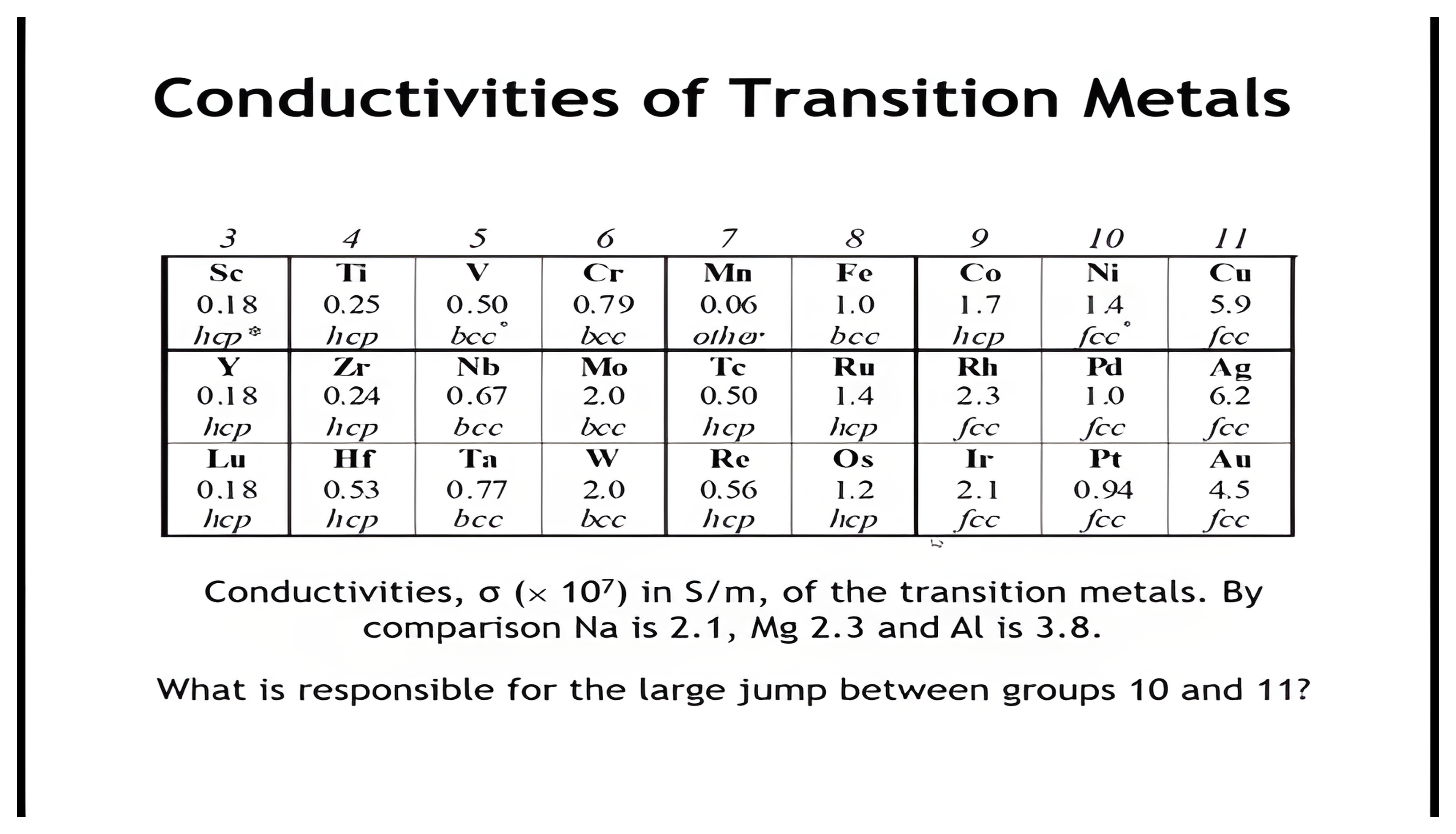
Conductivities of Transition Metals

Table of transition-metal conductivities in units of ten to the seventh siemens per meter across groups 3 through 11, with the coinage metals copper, silver, and gold jumping to 5.9, 6.2, and 4.5 while most transition metals sit far lower.

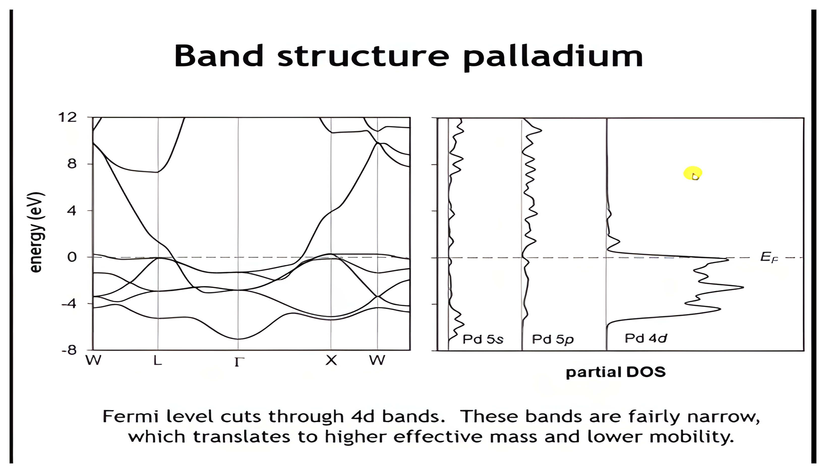
Band Structure of Palladium

The band structure of face-centered cubic palladium and its partial density of states: the Fermi level cuts through narrow 4d bands, which translates to higher effective mass and lower mobility.

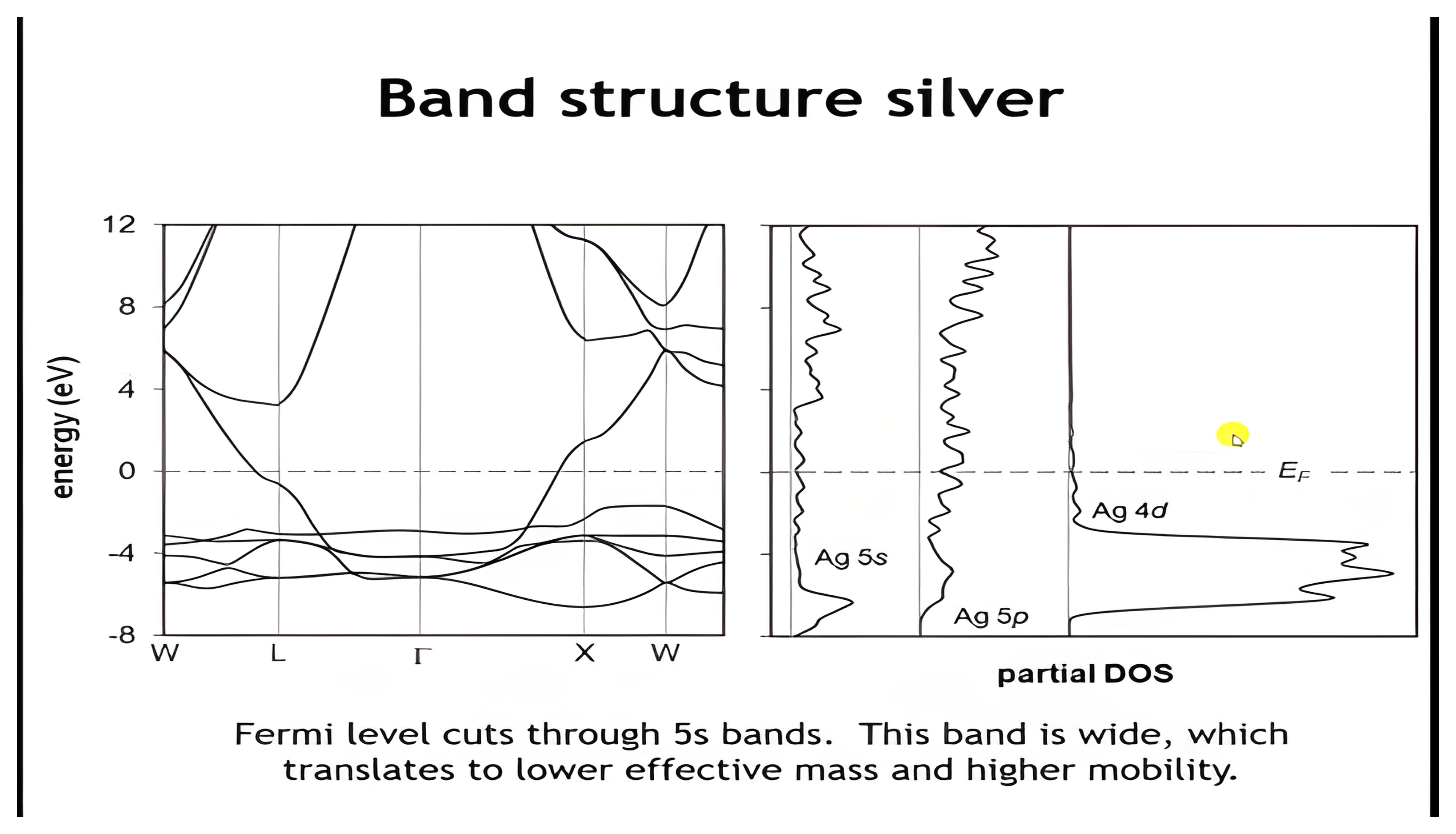
Band Structure of Silver

The band structure of face-centered cubic silver and its partial density of states: the filled 4d bands sit below the Fermi level, which now cuts through the wide 5s band, translating to lower effective mass and higher mobility.

Gradescope Quiz

Instruction to go to the Gradescope quiz.
CHEM 548