CHEM 548: Materials Chemistry

Lecture 13: Molecular Orbital Theory, Spin States, and Jahn–Teller Distortions

Mon 10/19/2026 · Meeting 15

Molecular orbitals from diatomics to transition-metal complexes, spin states, and Jahn–Teller distortions

Reading: Woodward, Karen, Evans, and Vogt, Solid State Materials Chemistry
Ch. 5 §5.3

Learning Objectives: Molecular Orbital Theory

Explain how atomic orbitals combine to form molecular orbitals.
Distinguish between bonding, antibonding, and nonbonding orbitals based on constructive and destructive interference.
Interpret simple MO diagrams (H₂, HeH⁺, O₂) and relate orbital overlap to bond order and stability.
Describe how orbital energy differences influence covalent, polar covalent, and ionic bonding character.
Understand σ vs. π interactions and how orbital symmetry governs overlap strength.
Recognize s–p mixing and its effect on molecular orbital energy ordering.
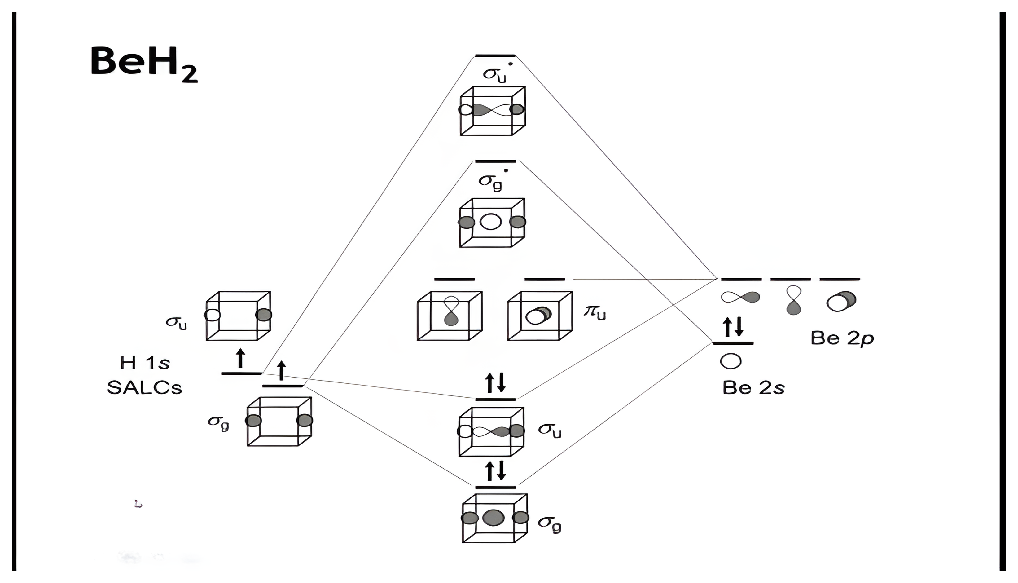
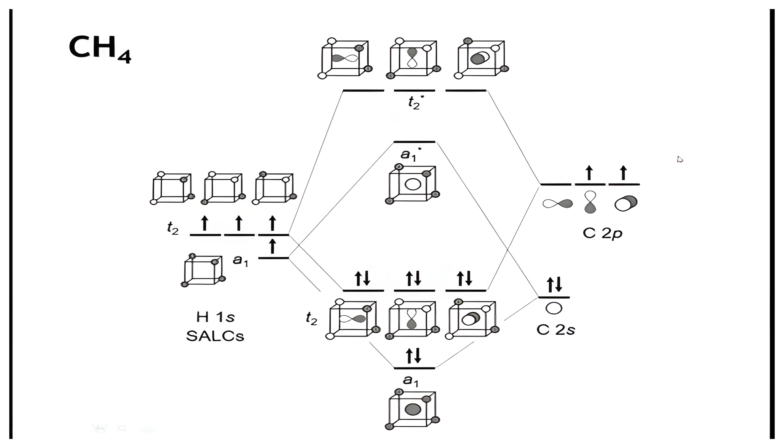
Apply the concept of symmetry-adapted linear combinations (SALCs) to polyatomic molecules (e.g., BeH₂, CH₄).
Define HOMO and LUMO and explain their importance in determining chemical reactivity.
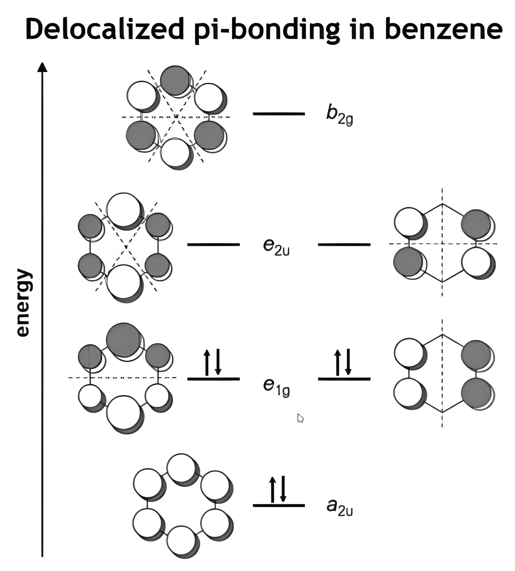
Identify how conjugated π systems (e.g., benzene) generate delocalized bonding and characteristic energy levels.

Molecular Orbitals

The electrons in an atom reside in atomic orbitals, each of which has a characteristic wavefunction.

When atoms combine to form molecules we need new orbitals, molecular orbitals, that have their own wavefunctions.

We will choose to describe molecular orbital wavefunctions as linear combination of atomic orbital wavefunctions (LCAO):

$\psi_{MO} = \sum c_1\psi_{AO(1)} + c_2\psi_{AO(2)} + \;...\,c_i\psi_{AO(i)}$

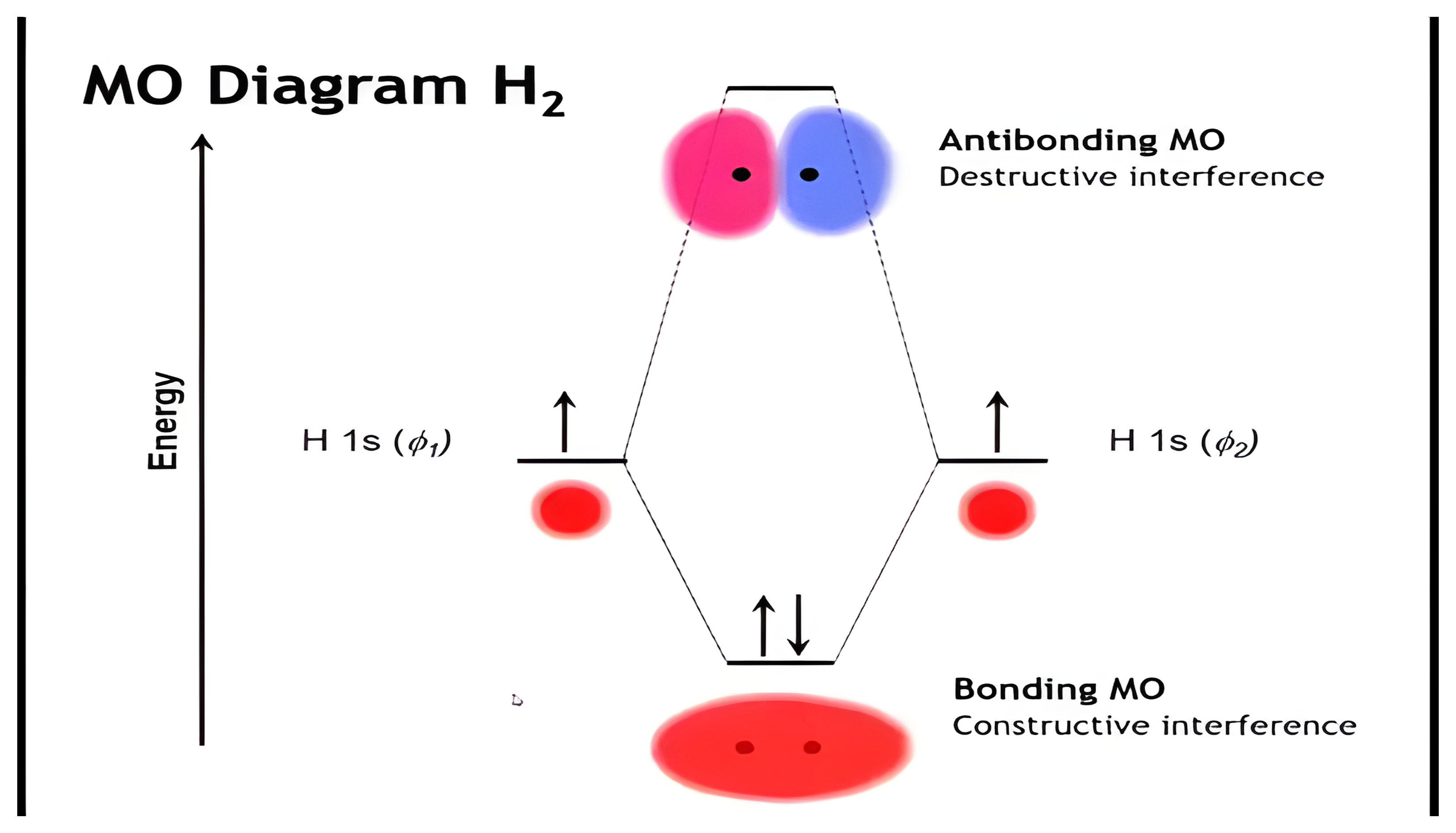
MO Diagram: H₂

MO diagram of H2 built from two hydrogen 1s orbitals: bonding and antibonding orbitals, then the antibonding MO circled, then the symbolic redraw with coefficients and energies of minus 17.6 and plus 4.2 electron volts.

The simplest and best-known molecular orbital diagram is for H₂.

Two MOs: a lower-energy bonding orbital and a higher-energy antibonding orbital
Bonding: constructive interference of the two 1s wave functions → more electron density between the nuclei
That density enhances attraction to the nuclei → stabilization: the bonding MO lies below the isolated atomic orbitals

[advance: circle the antibonding MO]

Antibonding: destructive interference; color = sign of the wave function, red positive, blue negative
Node between the atoms: zero electron density, electrons pushed out of the internuclear region → energy above the separate atoms

[advance: redraw with the symbolic orbitals and energies]

Symbolic style from here on: same sign → bonding; opposite signs → antibonding
Extended Hückel: bonding coefficients smaller than antibonding — the antibonding positive and negative regions partially cancel in the normalization integral, so the remaining portions scale up
Bonding stabilized ~4 eV; antibonding destabilized ~17 eV
Stabilization is always less than the destabilization → filling both orbitals provides no net stabilization, bond formation unfavorable

Let's look at those same two orbitals as wavefunctions along the bond axis.

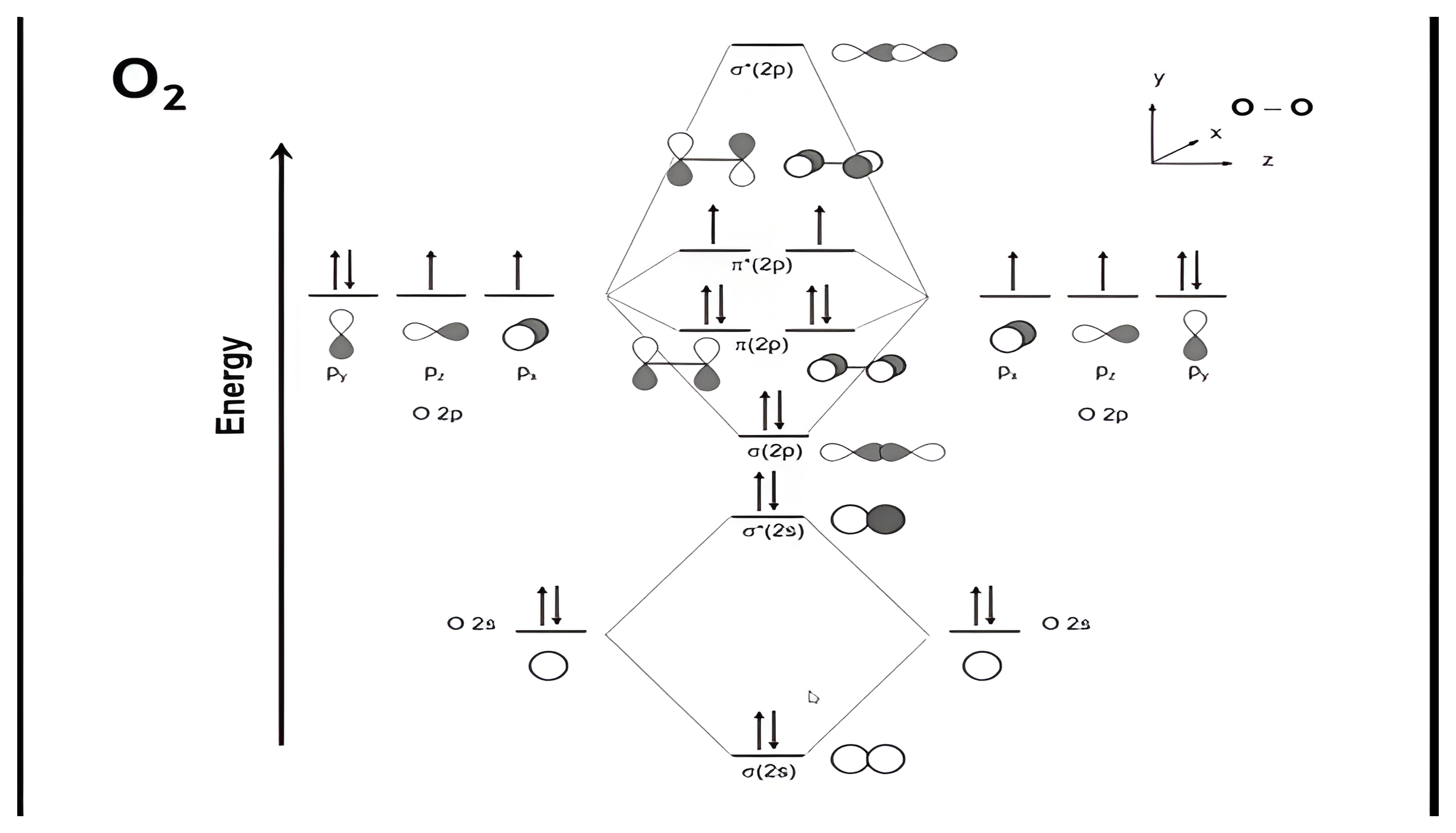
Molecular Orbital Wavefunctions

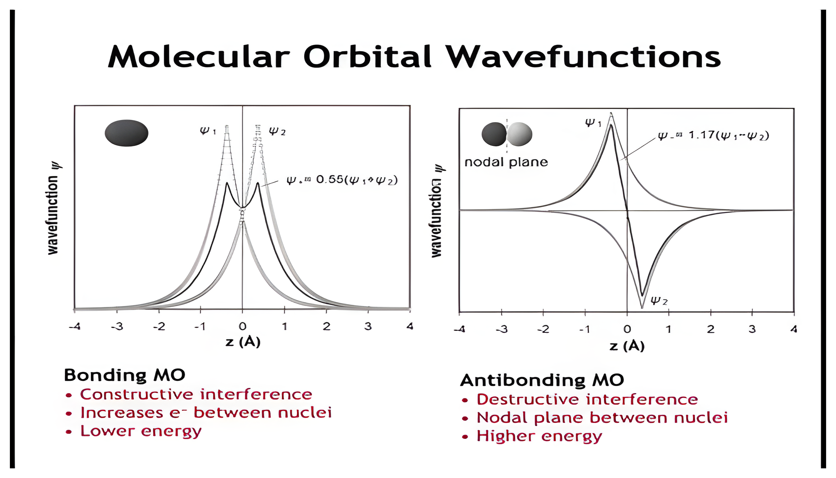
MO Diagram: HHe

MO diagram for the HHe molecule with unequal coefficients and energies, then a red mark highlighting the small stabilization of the bonding MO.

Now let’s look at a more complex case with two different atoms.

Helium’s higher nuclear charge → He 1s lower than hydrogen’s
The energy difference creates partial ionicity — what we call a polar covalent bond
Bonding MO: helium coefficient larger → resembles helium’s 1s more strongly; the antibonding is weighted toward hydrogen
As the gap grows: bonding resembles the more electronegative atom, antibonding the more electropositive; in the limit, purely ionic

[advance: mark the bonding-orbital stabilization]

Stabilization of the bonding MO decreases when the atomic orbitals differ in energy: H₂ ~4 eV, H–He only ~1.8 eV
Larger energy mismatch → overlap and mixing diminish → reduced bonding interaction

Next we move up to a real diatomic with p orbitals, O₂.

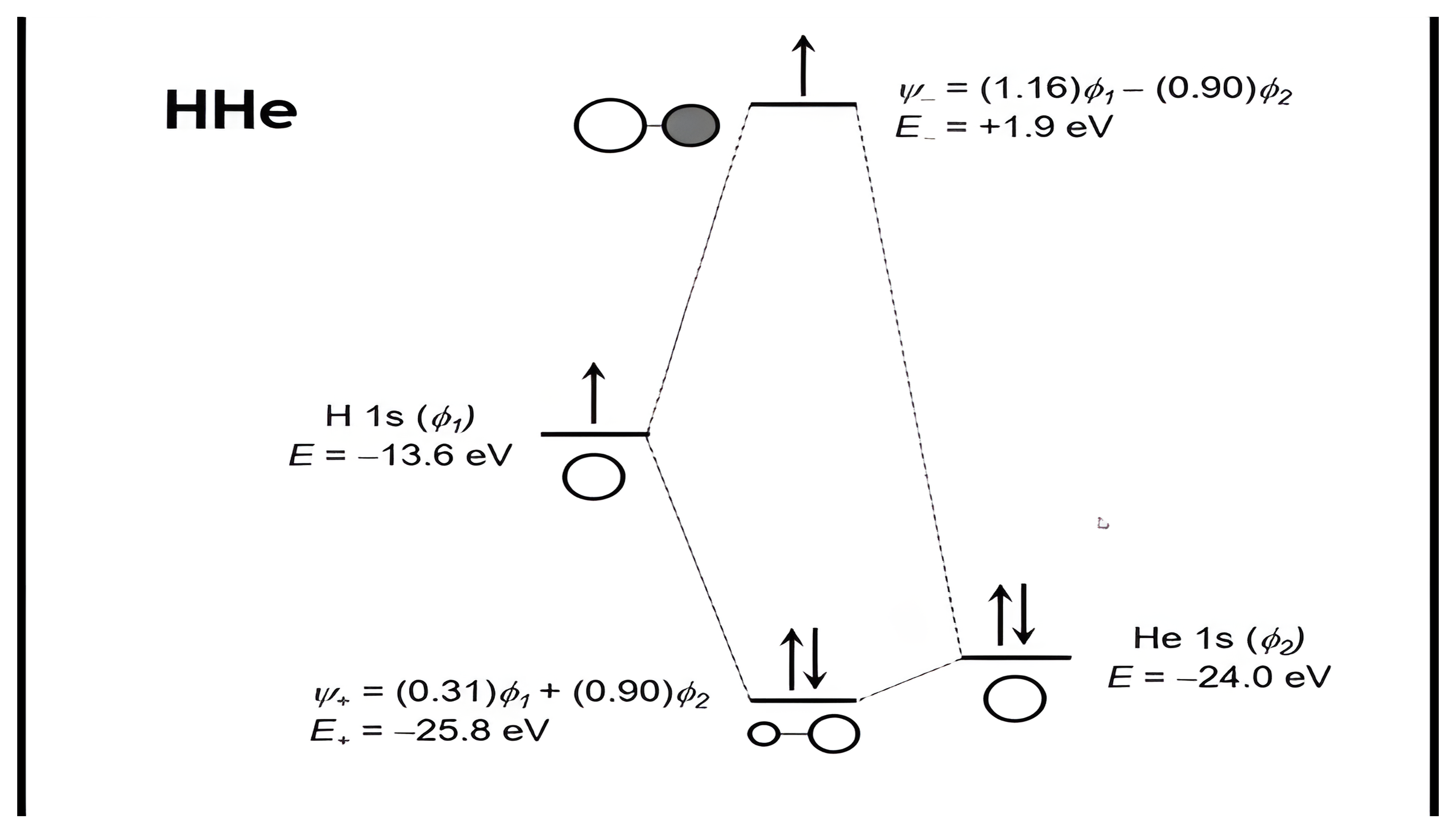
MO Diagram: O₂ and s–p Mixing

MO diagram of O2 with sigma and pi orbitals from the 2s and 2p sets, then the s-p mixing scheme for the sigma orbitals, then the corrected O2 diagram including s-p mixing.

Let’s examine O₂, starting with a simplified view and then moving toward the full MO diagram.

The two 2s overlap → bonding and antibonding MOs, similar to H₂; the 2p interactions split into a 1–2–2–1 pattern, not three equal pairs
p_z overlap head-on along z → σ bonding and antibonding; p_x, p_y side-on → π, with less overlap
Greater spatial overlap → larger bonding–antibonding gap → σ stronger than π
The true diagram must also account for σ–σ mixing between the 2s and 2p, which slightly alters energies and ordering

[advance: show the s–p mixing of the σ orbitals]

Adding the wave functions constructively → density between the nuclei → stabilizes; subtracting → density to the periphery → raises the energy
Mixing stabilizes the orbital with more 2s character, destabilizes the one with more 2p; same pattern for the σ antibonding orbitals

[advance: return to the O₂ diagram with the mixing included]

σ2s gains p character → stabilized; σ2p gains s character → destabilized; the antibonding orbitals shift the same way
Net effect: smaller σ2p–π2p gap; in lighter diatomics such as N₂ or C₂, mixing lifts σ2p above the π2p

To go beyond diatomics, we need a new tool: symmetry-adapted linear combinations.

Beyond Diatomics: SALCs

Table of central-atom s and p orbitals gaining ligand SALC columns: linear BeH2, then tetrahedral CH4, then octahedral SH6 grouped by nodal planes.

To move beyond diatomic molecules, we decompose the system into a central atom and its surrounding atoms, called ligands.

Group the ligand orbitals by symmetry into symmetry-adapted linear combinations (SALCs): how the ligand orbitals combine and interact with the central atom’s orbitals, consistent with the molecule’s overall symmetry

[advance: add the linear BeH₂ SALCs]

Symmetric SALC can overlap with the Be 2s; antisymmetric SALC aligns with the Be 2pₓ
The remaining 2p_y, 2p_z: no net bonding or antibonding overlap — these relationships can be derived formally from group theory, but here they are evident from visual inspection of orbital symmetry

[advance: add the tetrahedral CH₄ SALCs]

Methane: the four hydrogens form four ligand SALCs, each matching the symmetry of one of carbon’s valence orbitals
Totally symmetric SALC → carbon 2s; the other three → the three 2p → equivalent σ bonds in the tetrahedral geometry

[advance: add the octahedral SH₆ SALCs]

Octahedral hypothetical S–H₆: six ligands, one orbital each → six ligand SALCs; their shapes require group theory
First matches the sulfur s, next three align with the sulfur p; the remaining two have no matching symmetry → nonbonding

Let's put those SALCs to work and build the full MO diagram for BeH₂.

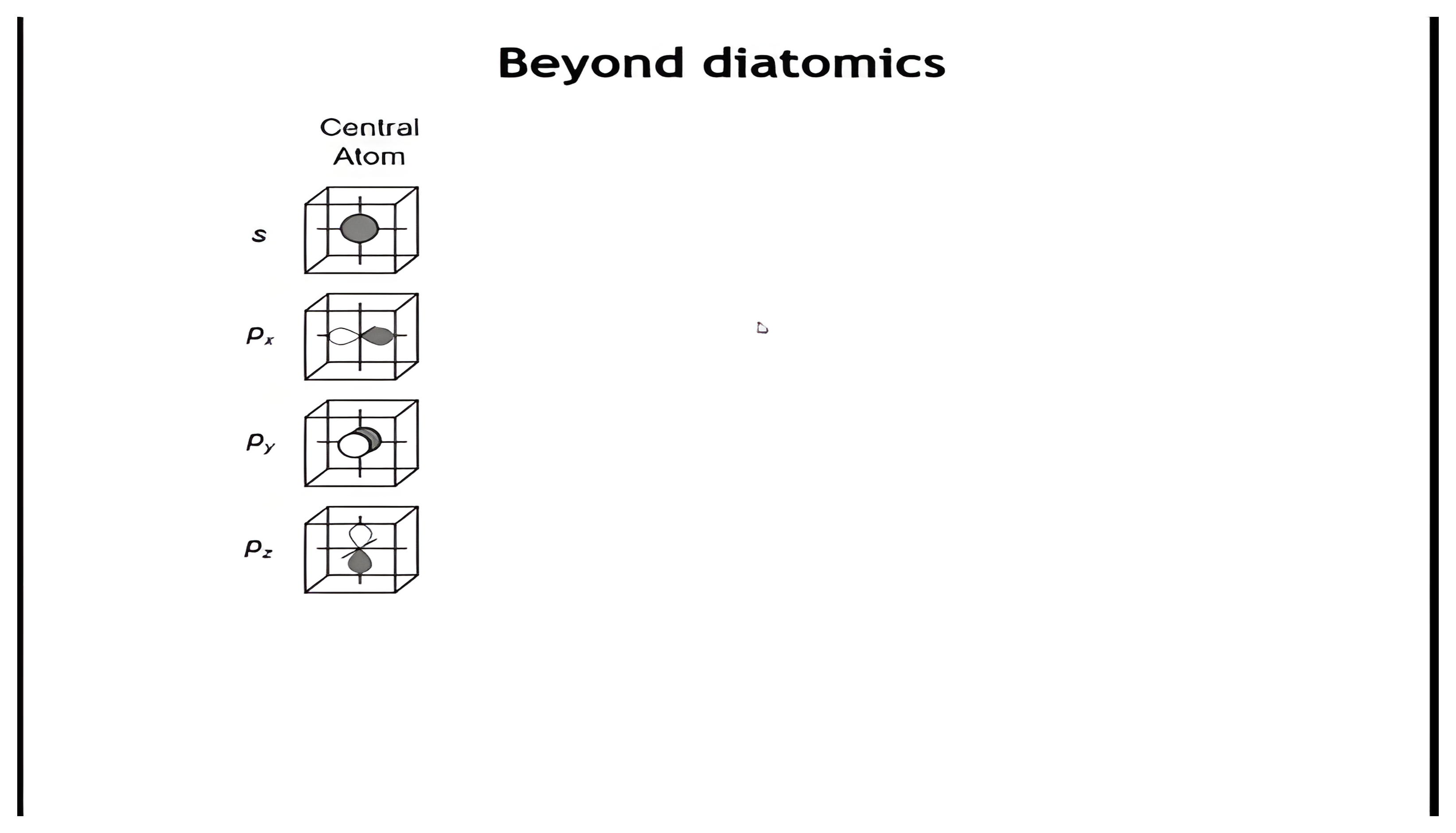
BeH₂: MO Diagram and Frontier Orbitals

MO diagram of BeH2 from hydrogen SALCs and beryllium 2s and 2p orbitals, then the HOMO and LUMO labels added.

In BeH₂, the ligand SALCs are shown on the left and the Be 2s and 2p orbitals on the right.

Electrons: Be contributes two in its 2s, the two hydrogens one each
Symmetric (σ_g) SALC + Be 2s → bonding and antibonding MOs; antisymmetric (σ_u) SALC + the axial Be 2p → another bonding/antibonding pair
2p above 2s → its MOs sit higher in energy
The two perpendicular Be 2p: no matching ligand SALCs → nonbonding, effectively like atomic orbitals

[advance: label the HOMO and LUMO]

Certain orbitals dominate a molecule’s behavior — the frontier orbitals: HOMO = highest occupied, LUMO = lowest unoccupied
BeH₂: HOMO = the Be 2p–hydrogen SALC bonding interaction; LUMO = the degenerate nonbonding Be 2p

Now let's do the same thing for methane.

CH₄: MO Diagram

MO diagram of methane from hydrogen 1s SALCs and carbon 2s and 2p orbitals, with a1 and t2 bonding and antibonding sets.

Delocalized $\pi$ Bonding in Benzene

The six pi molecular orbitals of benzene ordered by energy and nodal-plane count, from all-bonding a2u to all-antibonding b2g.

Summary — Molecular Orbital Theory

Molecular orbitals (MOs) form from linear combinations of atomic orbitals (LCAO); electrons are described by delocalized wave functions over the entire molecule.
Bonding MOs arise from constructive interference (increased electron density between nuclei → stabilization).
Antibonding MOs arise from destructive interference (nodal plane between nuclei → destabilization).
Energy splitting between bonding and antibonding orbitals increases with orbital overlap and decreases with energy mismatch.
Polarity arises when orbitals of unequal energy mix, giving partial ionic character.
σ and π bonds differ by overlap geometry: σ bonds form along the internuclear axis, π bonds form side-on.
s–p mixing alters MO energy ordering, notably in lighter diatomics (C₂, N₂).
For polyatomic molecules, ligand orbitals combine into SALCs that mix with central-atom orbitals of matching symmetry.
HOMO and LUMO define the frontier orbitals controlling reactivity and optical transitions.
In conjugated π systems, delocalization spreads bonding over many atoms, producing evenly spaced energy levels (e.g., benzene).

-Molecular orbitals form when we combine atomic orbitals—literally a linear combination of atomic orbitals, or LCAO.

Electrons no longer tied to a single atom: wave functions extend over the entire molecule
Bonding = constructive overlap, density between the nuclei, stabilization; antibonding = destructive, nodal plane, higher energy; larger overlap and smaller mismatch → bigger splitting
Unequal-energy mixing → polarity — one side takes on more character from the lower-energy orbital
σ along the internuclear axis, π side-on; s–p mixing can shift the order, as in C₂ and N₂
Polyatomics: ligand group orbitals or SALCs matching the central atom’s orbital symmetry
HOMO and LUMO: the frontier, controlling reactivity and optical transitions; conjugated π systems spread over the framework → delocalized bonding, evenly spaced levels, stability

Here is your homework for this part.

Check Your Understanding: $\sigma$–$\pi$ Splitting

Question asking how sigma-pi splitting differs for p orbitals in O2 and what determines the bonding-antibonding energy separation, then its answer.

Check Your Understanding: SALCs

Question asking what a symmetry-adapted linear combination is and how it simplifies MO construction in polyatomic molecules, then its answer.

Learning Objectives: MO Theory Part II

Understand how molecular orbital theory applies to transition metal complexes with octahedral and tetrahedral symmetry.
Identify which atomic orbitals on the metal and ligands participate in bonding interactions.
Construct ligand group orbitals (SALCs) for octahedral and tetrahedral complexes and determine which metal orbitals they can mix with.
Explain the formation of σ-bonding, π-bonding, and nonbonding molecular orbitals in metal–ligand systems.
Interpret how energy matching between metal and ligand orbitals governs bonding strength and orbital participation.
Describe the splitting pattern of d orbitals (t_2g/e_g in octahedral, e/t₂ in tetrahedral) and relate it to bonding interactions.
Compare the magnitude and direction of orbital splitting in octahedral vs. tetrahedral geometries.
Connect molecular orbital diagrams to crystal field theory concepts and identify the frontier orbitals relevant to reactivity.

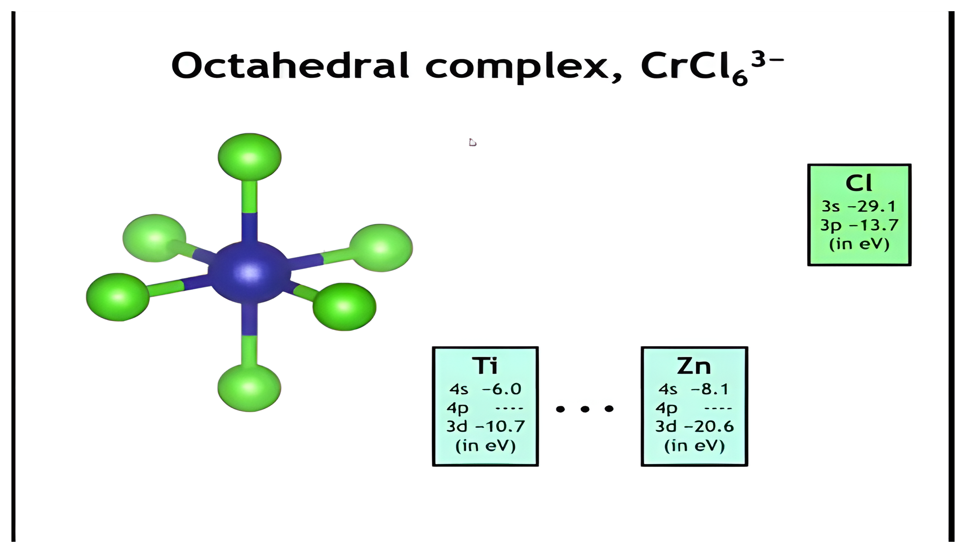
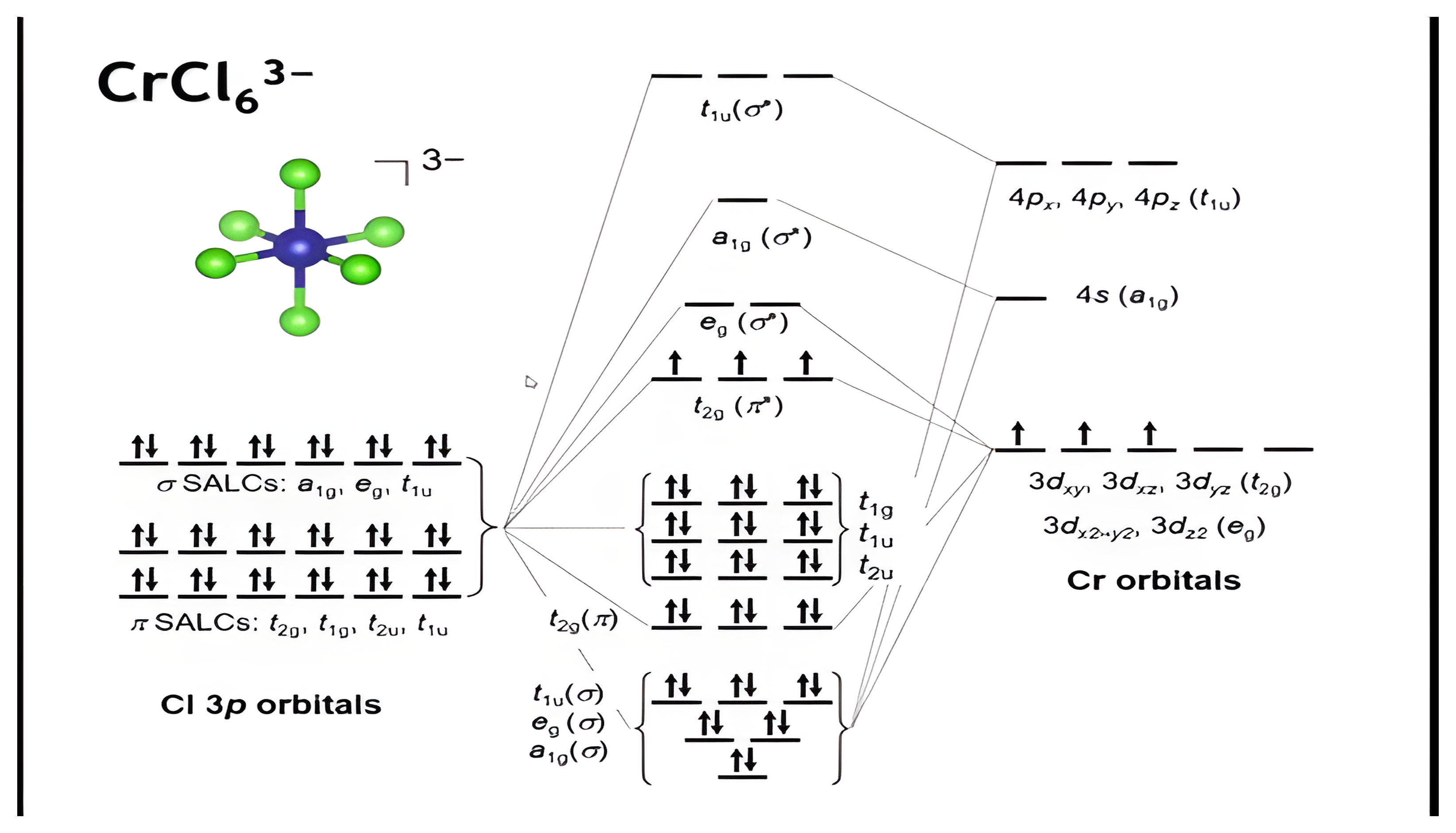
Octahedral Complex: CrCl₆³⁻

Ball-and-stick model of octahedral CrCl6 3- with chlorine, titanium, and zinc orbital energies, then the orbital counts: 18 chlorine 3p AOs and 5 Cr 3d, 1 Cr 4s, 3 Cr 4p AOs.

Let’s take chromium hexachloride (CrCl₆³⁻) as our model system.

First step: determine which atomic orbitals combine to form MOs — as in hydrogen–helium, orbitals interact most strongly when energies are similar
Chlorine 3s ~–29 eV; 3p ~–13 to –14 eV
Interpolating chromium between titanium and zinc: 3d near –12 to –13 eV — close to chlorine 3p; 4s and 4p higher
So we simplify to interactions between chlorine 3p and chromium 3d

[advance: count the valence orbitals]

Chlorine 3s treated as core, ignored; three 3p per chlorine, six chlorines → 18 chlorine 3p orbitals
Chromium: all nine valence orbitals — five 3d, one 4s, three 4p

Now let's count the electrons that go into this diagram.

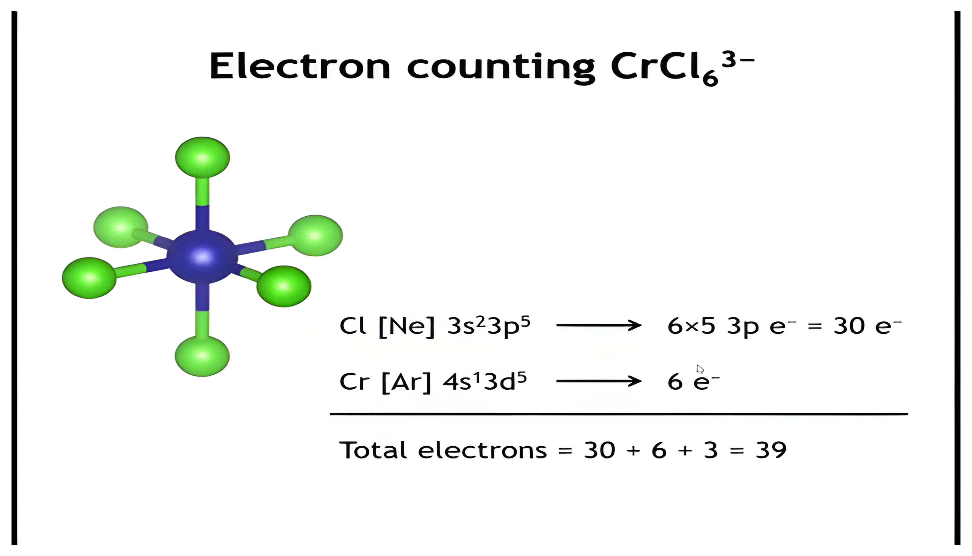
Electron Counting: CrCl₆³⁻

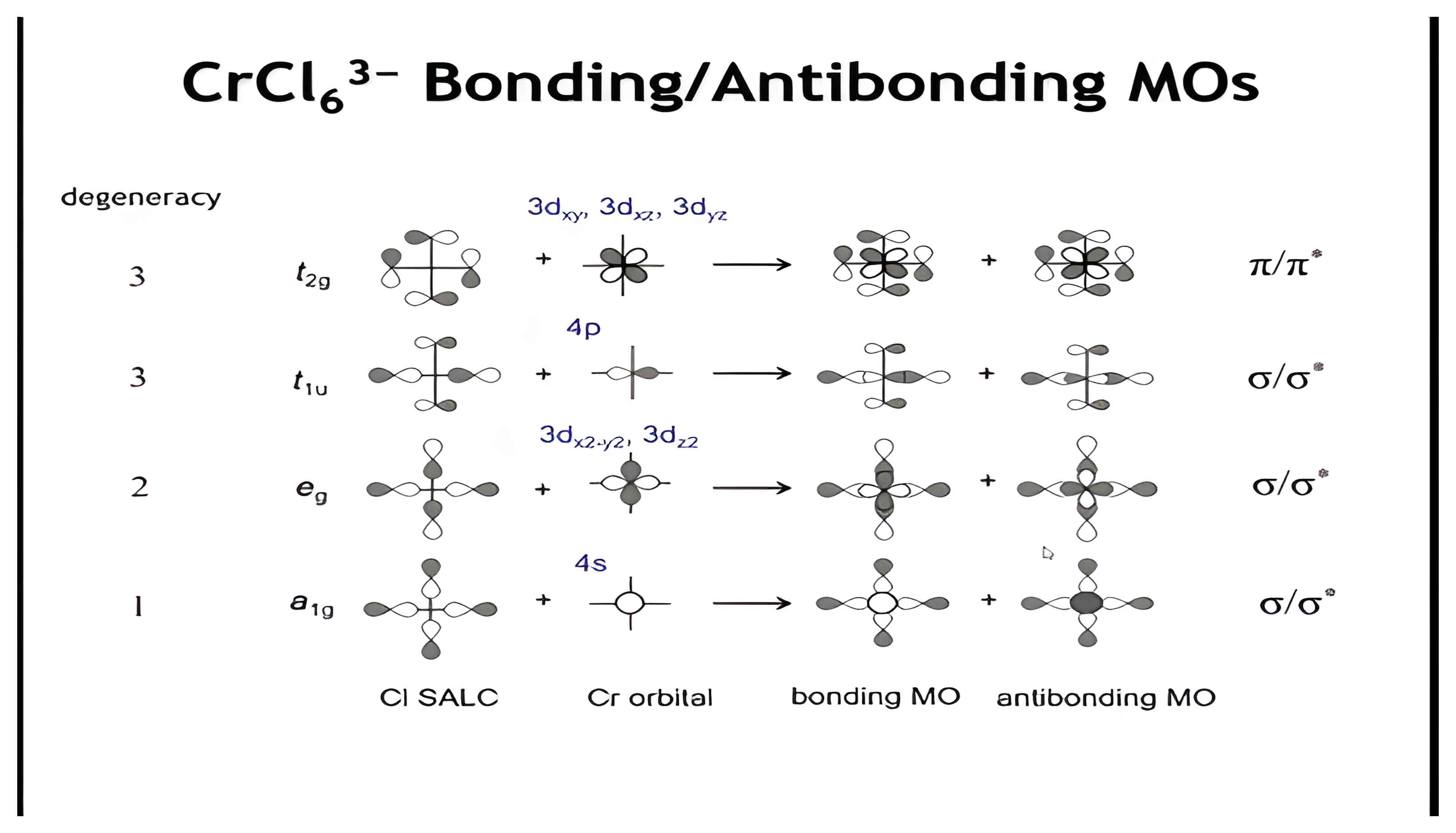
Electron counting for CrCl6 3-: 30 chlorine 3p electrons, 6 chromium valence electrons, and 3 from the charge, totaling 39.

CrCl₆³⁻: Bonding and Antibonding MOs

Chlorine SALCs paired with chromium orbitals by symmetry: t2g pi, t1u sigma with 4p, eg sigma with dx2-y2 and dz2, and a1g sigma with 4s, each forming bonding and antibonding MOs.

CrCl₆³⁻: Nonbonding MOs

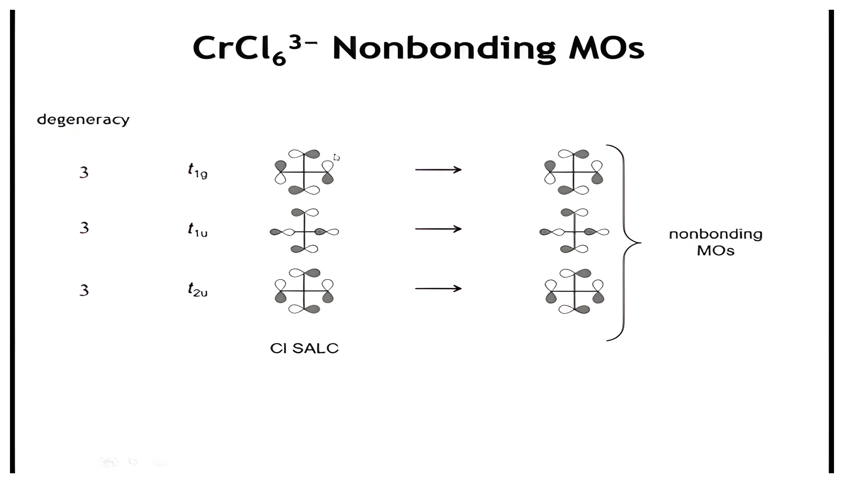
The t1g, t1u, and t2u chlorine SALCs that remain as nonbonding molecular orbitals.

The $t_{1u}$ SALCs share symmetry with the Cr $4p$ set, not the $3d$ orbitals. Per Solid State Materials Chemistry, §5.3.8.

CrCl₆³⁻: The Full MO Diagram

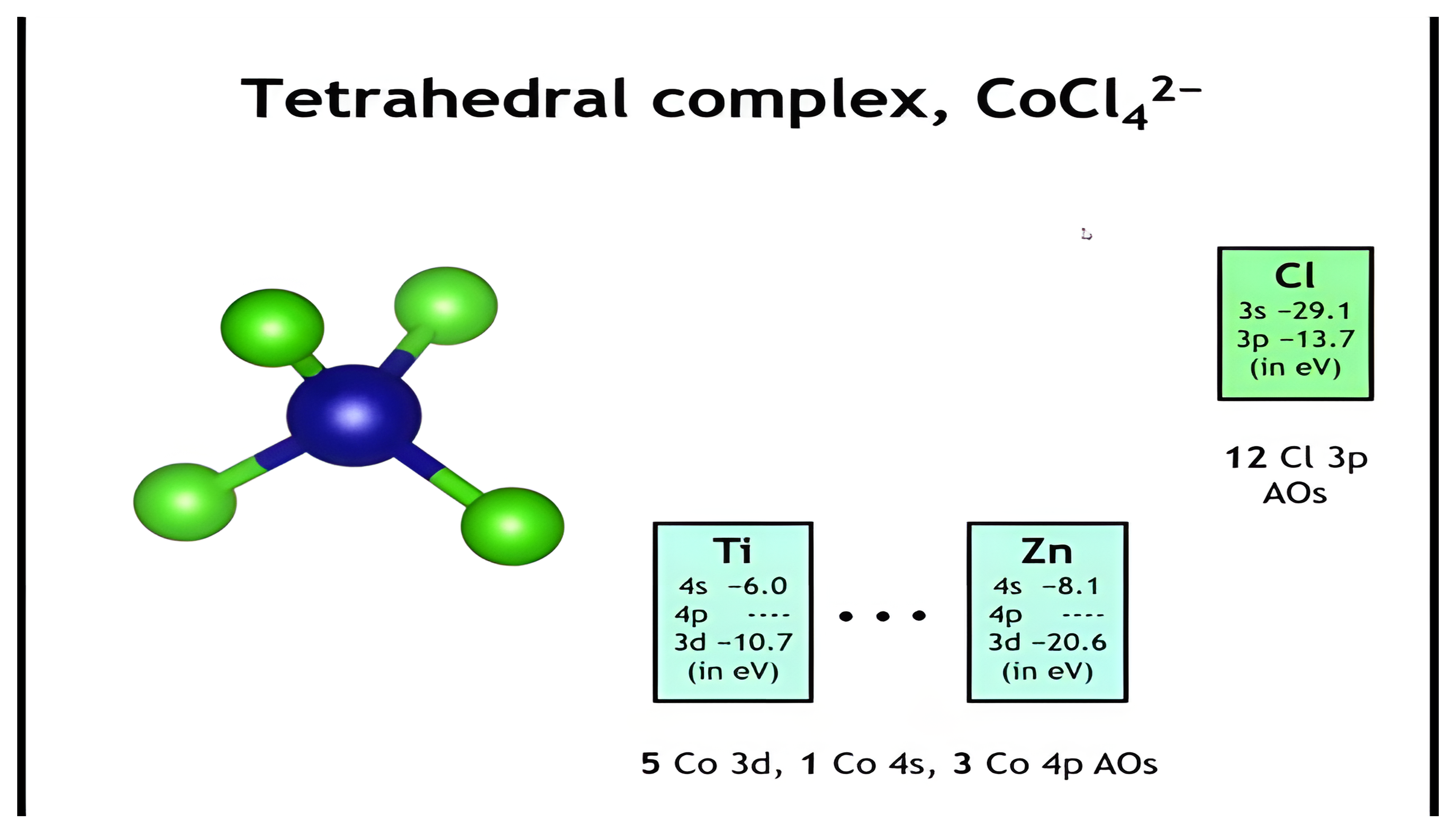
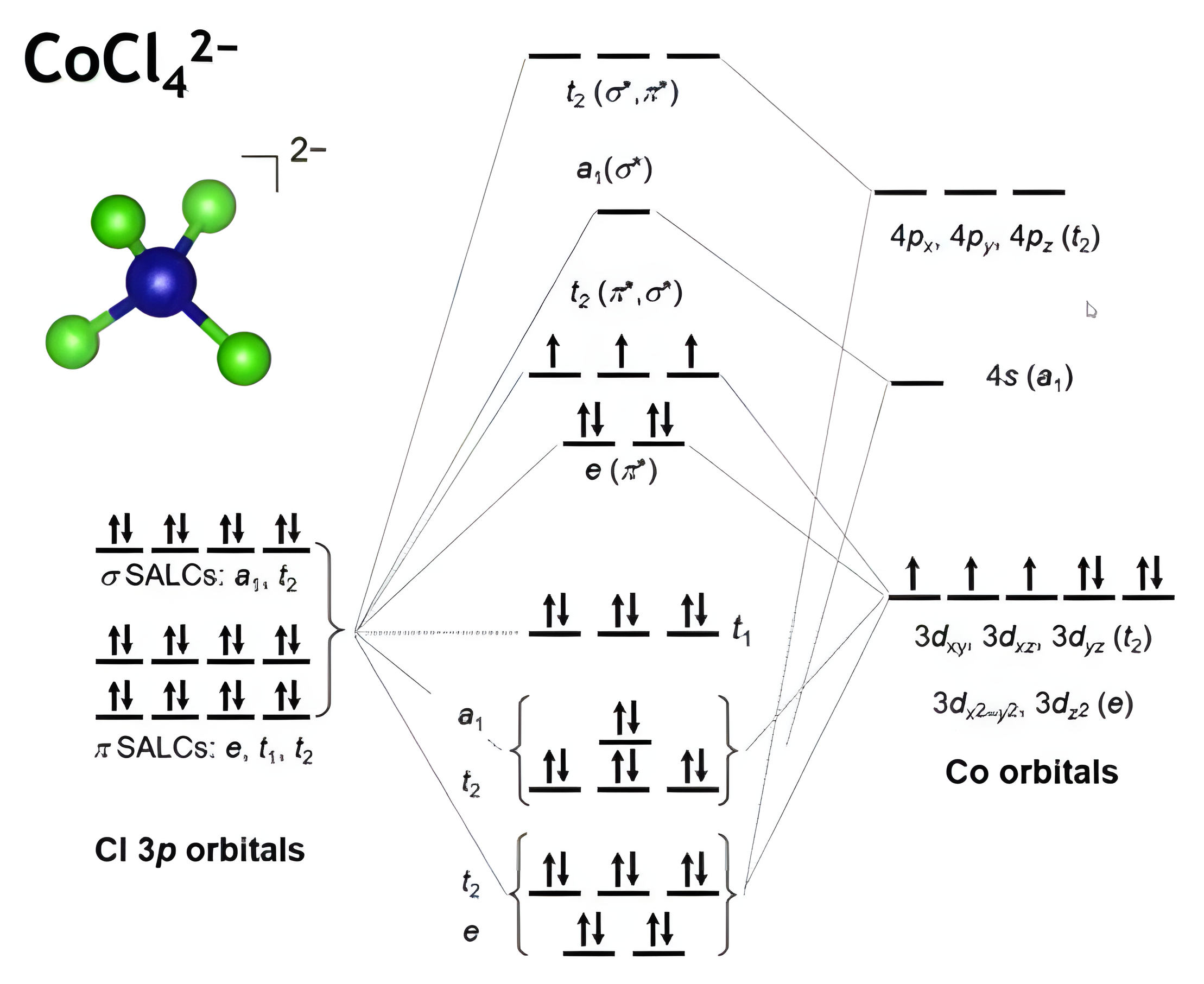
Full MO diagram of CrCl6 3- showing 9 bonding, 9 nonbonding, and 9 antibonding MOs with the t2g pi-star and eg sigma-star frontier orbitals.

Tetrahedral Complex: CoCl₄²⁻

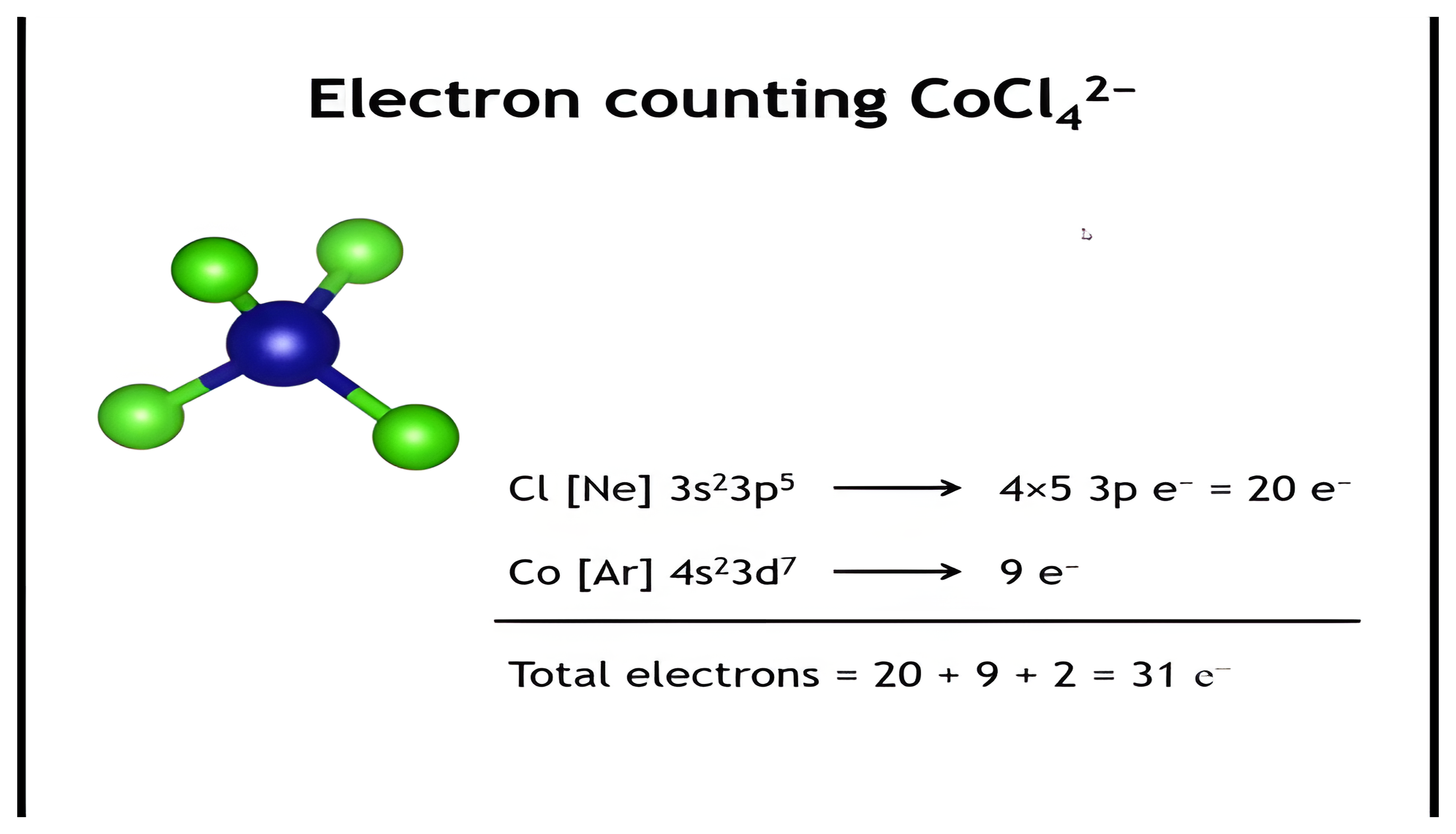
Ball-and-stick model of tetrahedral CoCl4 2- with chlorine, titanium, and zinc orbital energies and the orbital counts: 12 chlorine 3p AOs and 5 Co 3d, 1 Co 4s, 3 Co 4p AOs.

Electron Counting: CoCl₄²⁻

Electron counting for CoCl4 2-: 20 chlorine 3p electrons, 9 cobalt valence electrons, and 2 from the charge, totaling 31.

CH₄ Revisited

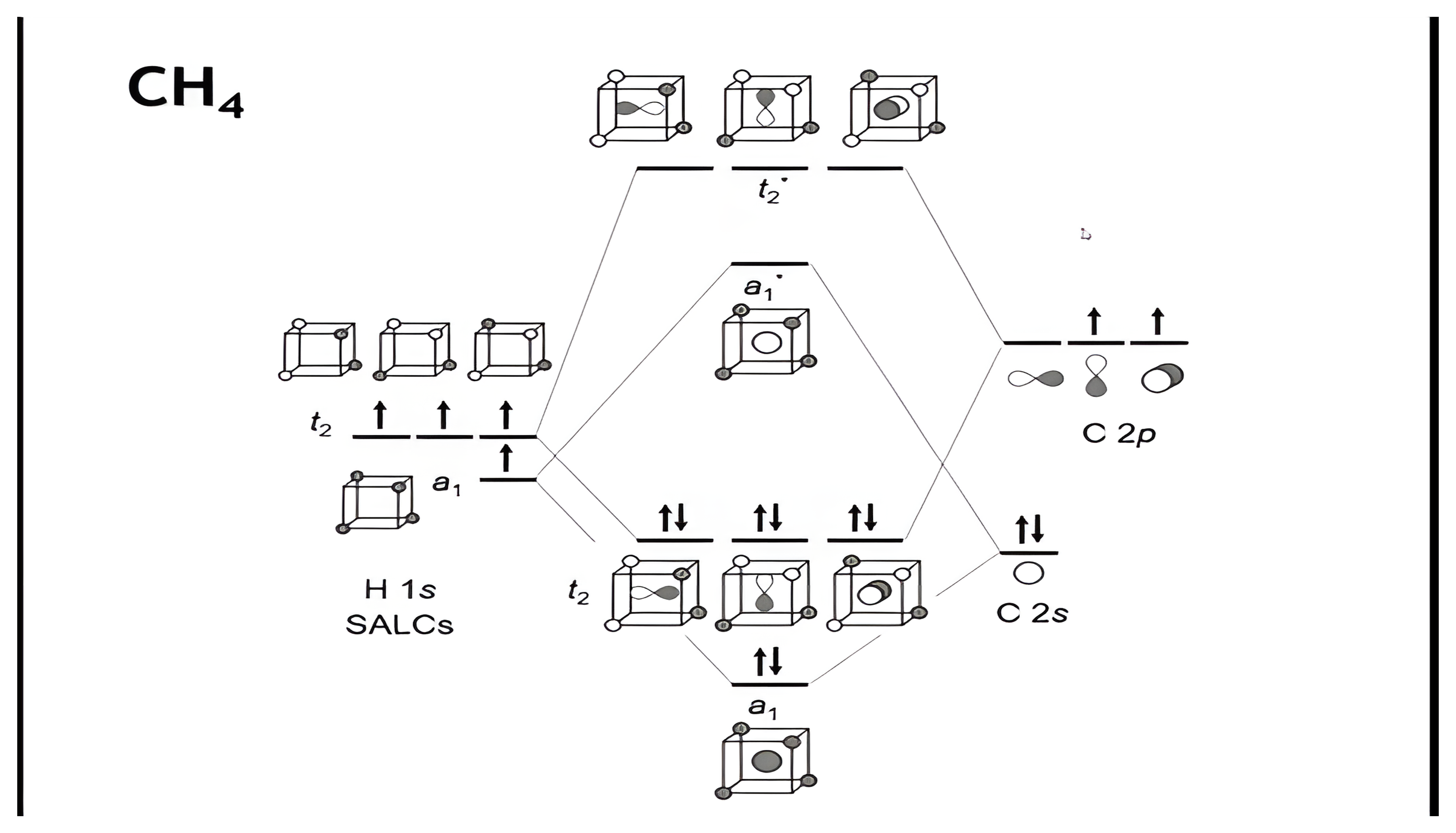
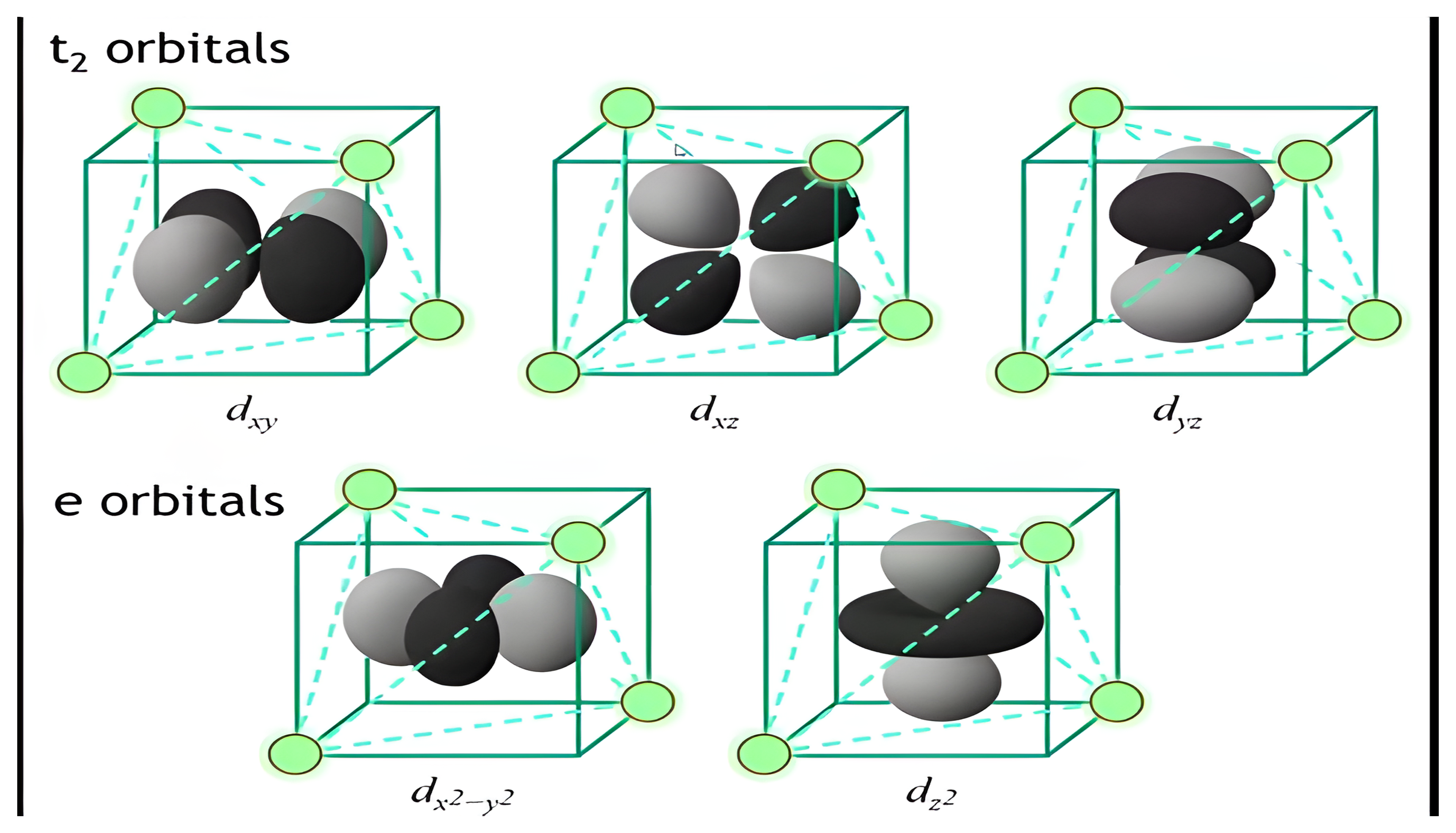
The methane MO diagram shown again as the template for the cobalt 4s and 4p interactions with the ligand SALCs.

The t₂ and e Orbitals in a Tetrahedron

The five cobalt d orbitals drawn inside a cube with ligands on alternating corners: the t2 set dxy, dxz, dyz and the e set dx2-y2 and dz2.

CoCl₄²⁻: The Full MO Diagram

Full MO diagram of CoCl4 2- with nine bonding, three nonbonding, and nine antibonding MOs; the e set lies below the t2 set.

Summary — MO Theory in Transition-Metal Complexes

[CrCl₆]³⁻ (Octahedral)

Orbitals: 9 metal (5 d, 1 s, 3 p) + 18 ligand (Cl 3p)
9 bonding, 9 antibonding, 9 non-bonding SALCs
Frontier orbitals:
- t₂g (dxy, dyz, dxz) = π antibonding (lower E)
- e_g (dx²−y², dz²) = σ antibonding (higher E)

[CoCl₄]²⁻ (Tetrahedral)

9 metal + 12 ligand orbitals → 9 bonding, 9 antibonding, 3 non-bonding
Splitting reversed: e (dx²−y², dz²) lower E; t₂ (dxy, dxz, dyz) higher E
Δ_t ≈ ½ Δ_o (no pure σ antibonding)

Takeaways

Geometry → symmetry → Δ magnitude and order.
Octahedral: t_2g below e_g | Tetrahedral: e below t₂
Frontier d-orbitals govern color and reactivity.

-Let’s summarize what we’ve done with molecular orbital theory applied to transition-metal complexes.

Octahedral [CrCl₆]³⁻: nine chromium valence orbitals + eighteen ligand 3p → nine bonding, nine antibonding, nine non-bonding combinations
The orbitals that matter most: antibonding with metal d character — t₂g π-antibonding, lower; e_g σ-antibonding, higher — the crystal-field splitting, t₂g below e_g
Tetrahedral [CoCl₄]²⁻: four ligands, twelve ligand 3p; the e orbitals interact least → lower, the t₂ set interacts more strongly → higher — ordering reversed
Δ_t roughly half of Δ₀: smaller overlap with ligands, fewer σ interactions
Takeaway: geometry and symmetry control both the order and the size of the splitting; the frontier antibonding d-orbitals govern optical properties, magnetism, and reactivity

Now test yourself on the two field-splitting patterns.

Check Your Understanding: Field Splitting

Question comparing FeCl6 4- octahedral and FeCl4 2- tetrahedral for oxidation state, d-electron count, splitting pattern, and unpaired electrons, then the worked answer.

Question, on field splitting. For chloride ligands, weak field, compare [FeCl₆]⁴⁻, octahedral, and [FeCl₄]²⁻, tetrahedral. Determine the iron oxidation state, the d-electron count, the orbital splitting pattern, and the number of unpaired electrons. Identify which has the larger splitting and explain why. Take a moment and work it through.

[advance: reveal the answer]

Each chloride is minus one: [FeCl₆]⁴⁻, x minus 6 equals minus 4 → iron 2+, 3d⁶; [FeCl₄]²⁻, x minus 4 equals minus 2 → again 2+, 3d⁶
Octahedral: t₂g lower, e_g higher; weak field → high spin, t₂g⁴ e_g², four unpaired electrons
Tetrahedral: e lower, t₂ higher; weak field → high spin, e³ t₂³, four unpaired electrons
Δ_t about half of Δ_o; octahedral larger because the ligands point directly at the metal orbitals, a stronger σ interaction
So both high-spin Fe²⁺, d⁶, four unpaired; [FeCl₆]⁴⁻ has the larger splitting

Here is the homework problem for this part.

Spin States & Jahn–Teller Distortions

Explain spin-state configurations
- Define high-spin and low-spin complexes.
- Relate crystal field splitting energy (Δ) and spin pairing energy (P).
- Predict spin states from ligand type (spectrochemical series) and metal identity (3d vs 4d/5d).
Compare structural preferences of d⁸ ions
- Describe why Ni²⁺ forms octahedral (rock salt) structures while Pt²⁺ forms square planar (Cooperite-type).
- Interpret orbital splitting diagrams for square planar fields.
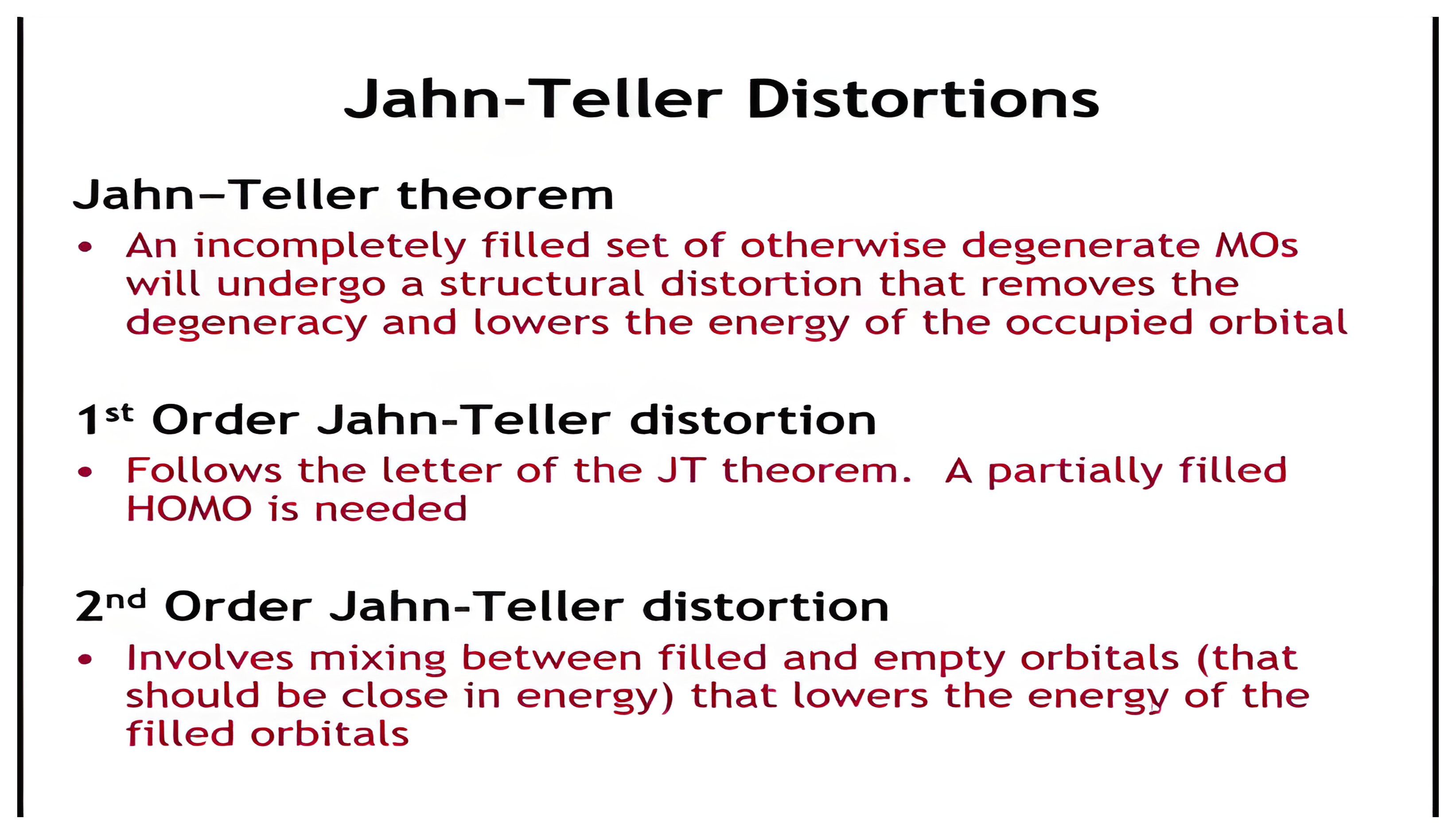
Apply the Jahn–Teller theorem
- Identify cases where electronic degeneracy causes structural distortion (e.g., high-spin d⁴, d⁹).
- Distinguish between elongated and compressed octahedra and the electronic rationale for each.
Describe second-order Jahn–Teller distortions
- Explain how HOMO–LUMO mixing stabilizes asymmetric geometries (e.g., NH₃, PbO).
- Recognize “stereoactive lone pair” distortions in s² cations (Pb²⁺, Bi³⁺).

Low-Spin and High-Spin Configurations

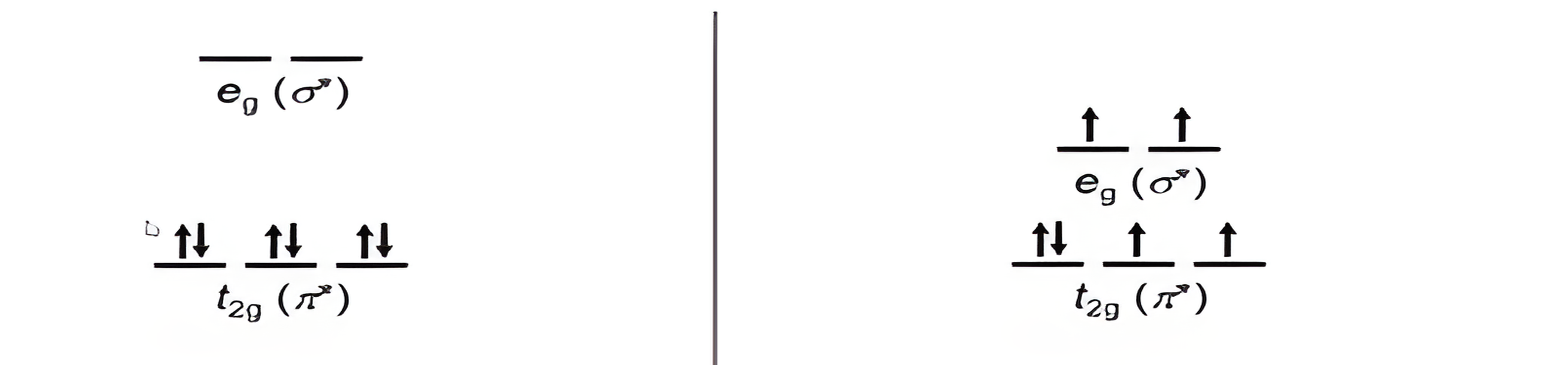
Left, all six electrons paired in the t2g set; right, three t2g electrons unpaired and two more in the eg set. Advancing swaps in the textbook spin-up and spin-down channel diagrams with the Delta and P energy spans marked.

low-spin configuration (P < Δ) high-spin configuration (P > Δ)

Δ = Crystal field splitting energy

Favors filling lower energy set (t_2g) of orbitals completely before adding electrons to higher energy set (e_g)

P = Spin pairing energy

Favors spreading the electrons out across all five d-orbitals before placing two electrons in the same orbital (strong Hunds rule coupling)

When transition metal ions form complexes, the frontier orbitals governing their properties are usually the metal’s d orbitals.

Octahedral field: lower t₂g (dxy, dyz, dxz), triply degenerate; higher e_g (dx²–y², dz²), doubly degenerate
Electrons fill t₂g first, singly with parallel spins per Hund’s rule
Fourth electron onward, two options: pair within t₂g or occupy the higher e_g; pairing costs spin-pairing energy P, promoting costs crystal field splitting Δ
P < Δ: pair in t₂g before e_g → low-spin; P > Δ: all five d singly before pairing → high-spin

[advance: show the spin-up and spin-down channels]

Textbook diagrams: two sets of five d-orbital lines, spin-up and spin-down
P < Δ: pair in the lower t₂g before e_g — low spin; P > Δ: fill all spin-up t₂g and e_g before any spin-down pairing — high spin

Next, let's look at the trends that control whether delta or P wins.

High spin vs. Low spin

2^nd and 3^rd row transition-metal ions adopt LS configurations
- The 4d and 5d orbitals interact more strongly with the ligands, increasing Δ, plus their larger size decreases P.
Increasing the covalency of the metal–ligand bonds increases Δ thereby favoring LS configurations
- Either by increasing the metal oxidation state or by moving from left to right across the transition-metal series
Tetrahedrally coordinated ions are nearly always high spin
- Δ_tetr < Δ_oct
High field ligands (see spectrochemical series) favor LS configurations

I⁻ < Br⁻ < S²⁻ < Cl⁻ < F⁻ < C₂O₄²⁻ < H₂O < NH₃ < CN⁻ < CO

weak field strong field

Whether a complex adopts a high- or low-spin configuration depends on the relative magnitudes of crystal field splitting (Δ) and spin-pairing energy (P).

4d and 5d ions: larger d orbitals, more ligand overlap → larger Δ, smaller P — these ions are always low spin
Increasing metal–ligand covalency (shorter bond distance, higher metal electronegativity) also increases Δ → favors low spin
Tetrahedral fields: Δ about half the octahedral value → almost always high spin
Spectrochemical series: weak-field ligands like halides → small Δ, high spin; strong-field CO or CN⁻, with empty π* orbitals stabilizing t₂g levels → large Δ, low spin

Now let's watch these rules play out in two group-10 oxides, nickel oxide and platinum oxide.

Crystal Chemistry of Group 10 Monoxides

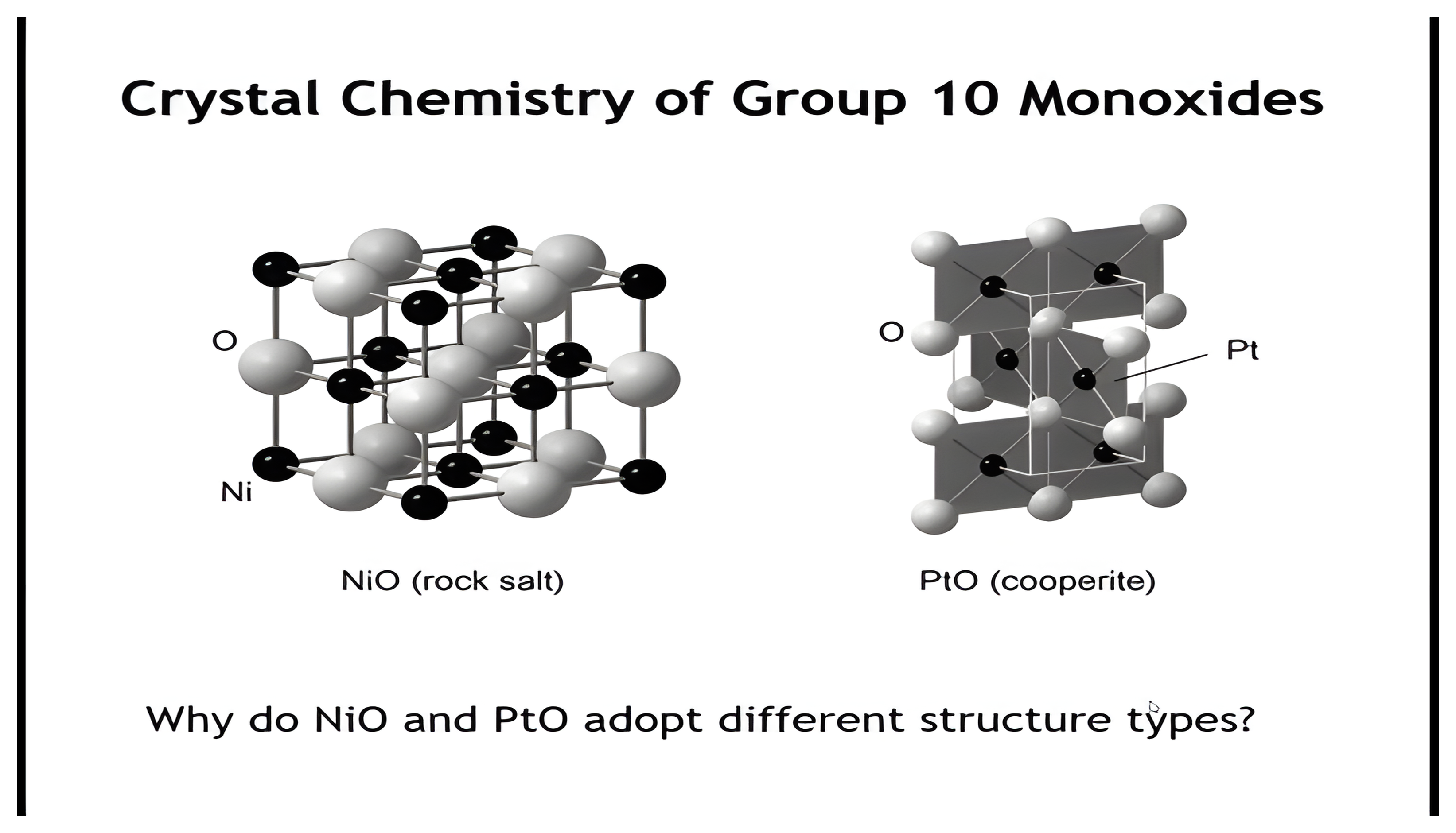
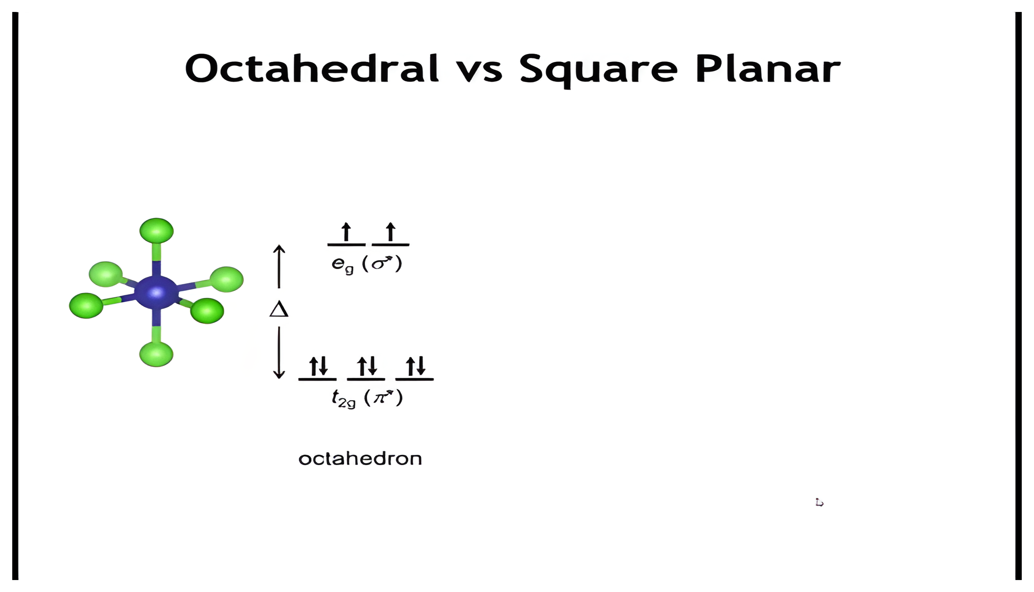
NiO in the rock-salt structure next to PtO in the cooperite structure, asking why the two group-10 monoxides adopt different structure types.

Octahedral vs. Square Planar

Octahedral d8 splitting diagram for NiO, then the correlation to the square-planar splitting that stabilizes PtO.

To understand this, examine how the 3d orbitals fill.

Octahedral field, Ni²⁺ in nickel oxide: eight 3d electrons — lower t₂g first, then the higher e_g
Now consider how this filling changes in a square-planar field

[advance: show the square-planar splitting]

Removing the z-axis ligands: x–y ligands move closer → d_xz, d_yz drop (less antibonding), d_xy rises (lobes in the ligand plane)
e_g splits further: d_z² lowers significantly, even below d_xy; d_x²–y², pointing directly at ligands, rises sharply
Result: one high-energy antibonding d_x²–y² and four lower orbitals; a d⁸ configuration stabilizes the square-planar field by filling the low orbitals and leaving d_x²–y² empty, though all electrons are now paired, increasing repulsion
Ni²⁺ (3d⁸): small splitting → octahedral, avoiding pairing energy; Pt²⁺ (5d⁸): strong metal–ligand interactions, large splitting → square-planar distortion, lowering d_z² and depopulating d_x²–y²
Square-planar coordination thus commonly appears for d⁸ and sometimes d⁹ ions with strong ligand fields

That electronic driving force for distortion has a general name: the Jahn-Teller theorem.

Jahn–Teller Distortions

The Jahn-Teller theorem with definitions of first-order and second-order distortions.

First-Order Jahn–Teller Distortion

A first-order Jahn–Teller distortion commonly occurs in octahedral complexes with high-spin d⁴ (e.g., Mn³⁺) or d⁹ (e.g., Cu²⁺) configurations.

e_g unevenly occupied — such as one electron shared between dz² and dx²–y² → a degenerate partially filled HOMO
The degeneracy drives the system to distort and lower its symmetry, stabilizing one orbital and reducing total energy

[advance: show the compressed octahedron]

Distortion removes the degeneracy, as the theorem predicts — though the theorem doesn’t specify how; two main distortions are possible
Compressed octahedron: z-axis bonds shorten, xy-plane bonds lengthen → dz² rises, dx²–y² lowers
Both are σ-antibonding, but compression reduces the antibonding character of dx²–y², stabilizing it and lowering the overall energy

[advance: show the elongated octahedron]

We could also elongate: stretch the z-axis bonds, compress the xy-plane — the opposite distortion of the compressed case
Both lower the energy by a similar amount → from the orbital diagram alone, unclear which will occur
In practice, high-spin d⁴ or d⁹ complexes almost always adopt the elongated octahedral geometry; compressed is rare — the question is what stabilizes the elongated structure

The real copper and mercury halides tell us which distortion nature picks.

Distortions in d⁹ and d¹⁰ Halides

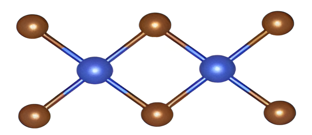
Copper bromide chain: each blue copper ion carries four short bonds to bridging bromides and two longer axial bonds.

CuBr₂ distances
4×2.41 Å, 2×3.15 Å

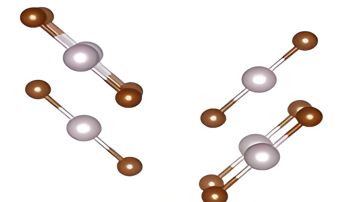
Mercury bromide: near-linear two-short-bond units stacked so the remaining four bromide contacts are much longer.

HgBr₂ distances
2×2.45 Å, 4×3.24 Å

Cu²⁺ (d⁹) ions almost always take the 2 long + 4 short distortion (elongated octahedron)

d¹⁰ ions, such as Hg²⁺ adopt very large 2 short + 4 long distortions (compressed octahedron).

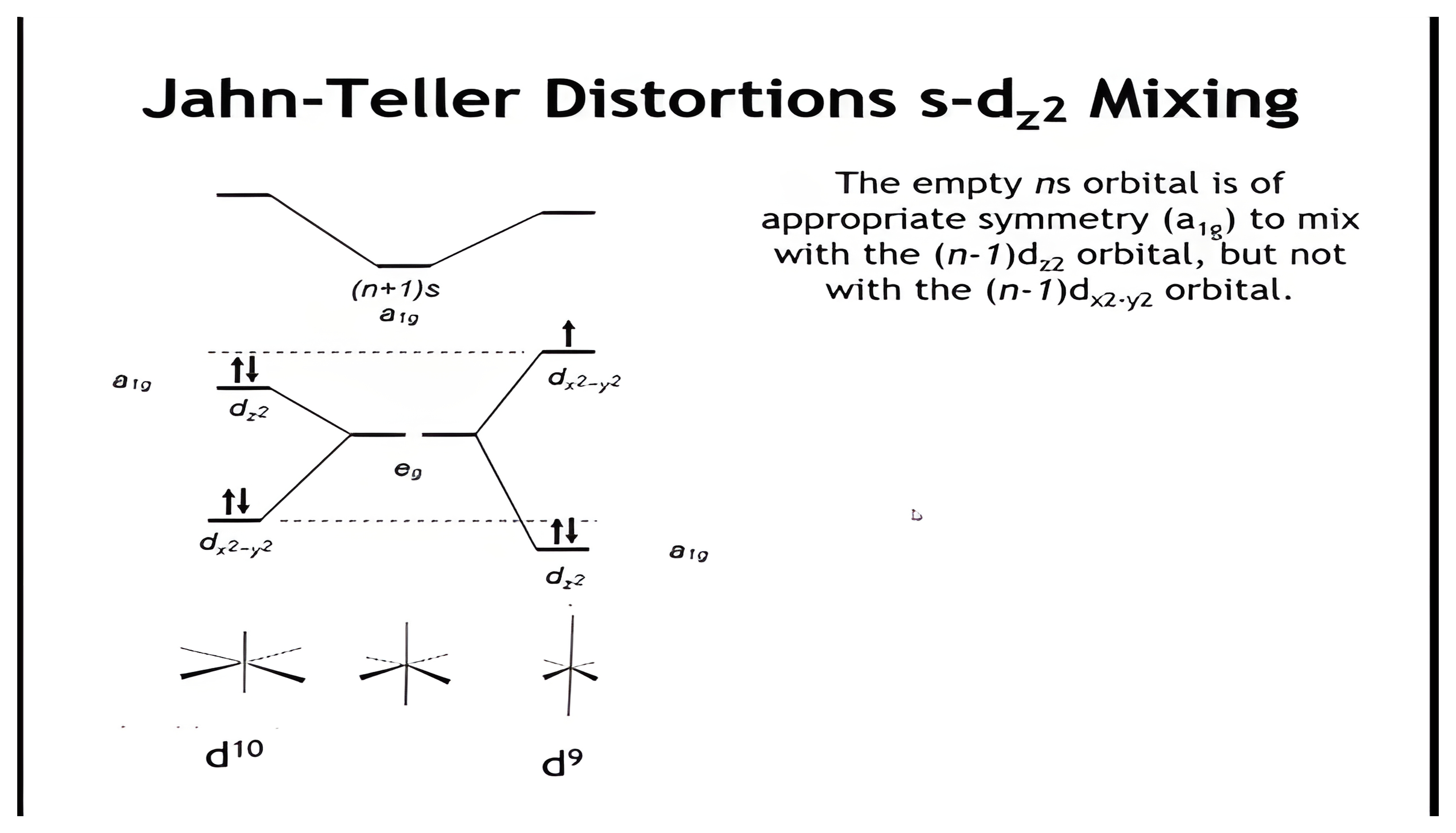
Why is this so? Why do d¹⁰ ions distort at all?

Jahn–Teller Distortions: s–d_z² Mixing

Molecular-orbital diagram for s and d z squared mixing in distorted octahedra, then the annotated d9 copper case, then the d10 mercury case.

To explain this, we need to include the nearby empty s orbital—4s for Cu²⁺ or 6s for Hg²⁺.

Undistorted octahedron: the metal’s e₉ orbitals (dz², dx²–y²) degenerate, E_g symmetry; the s orbital A₁g — different symmetries, no mixing
Distorting (either elongating or compressing) lowers the symmetry from O_h to D₄h (Hermann–Mauguin 4/mmm) → previously forbidden mixing becomes allowed, changing relative energies

[advance: show the d⁹ case]

Lowered symmetry: dz² gains A₁g symmetry, matching the s orbital → the two can mix (hybridize), just like σ(s) and σ(p) mixing in O₂
The interaction raises the s orbital and lowers dz²
d⁹: elongation lowers dz² enough that it becomes doubly occupied, dx²–y² singly → greater stabilization than compression would give; s–dz² hybridization under elongation explains the preferred d⁹ distortion

[advance: show the d¹⁰ case]

d¹⁰ (e.g., Hg²⁺): both dz² and dx²–y² doubly occupied → favorable to raise dz² toward the s orbital, increasing s–dz² hybridization
Greater hybridization strengthens the mixing and stabilizes dz² overall
The opposite distortion would widen the dz²–s gap → less hybridization, less stabilization; so compression increases s–dz² overlap and lowers total energy

The cleanest example of this second-order mixing is ammonia.

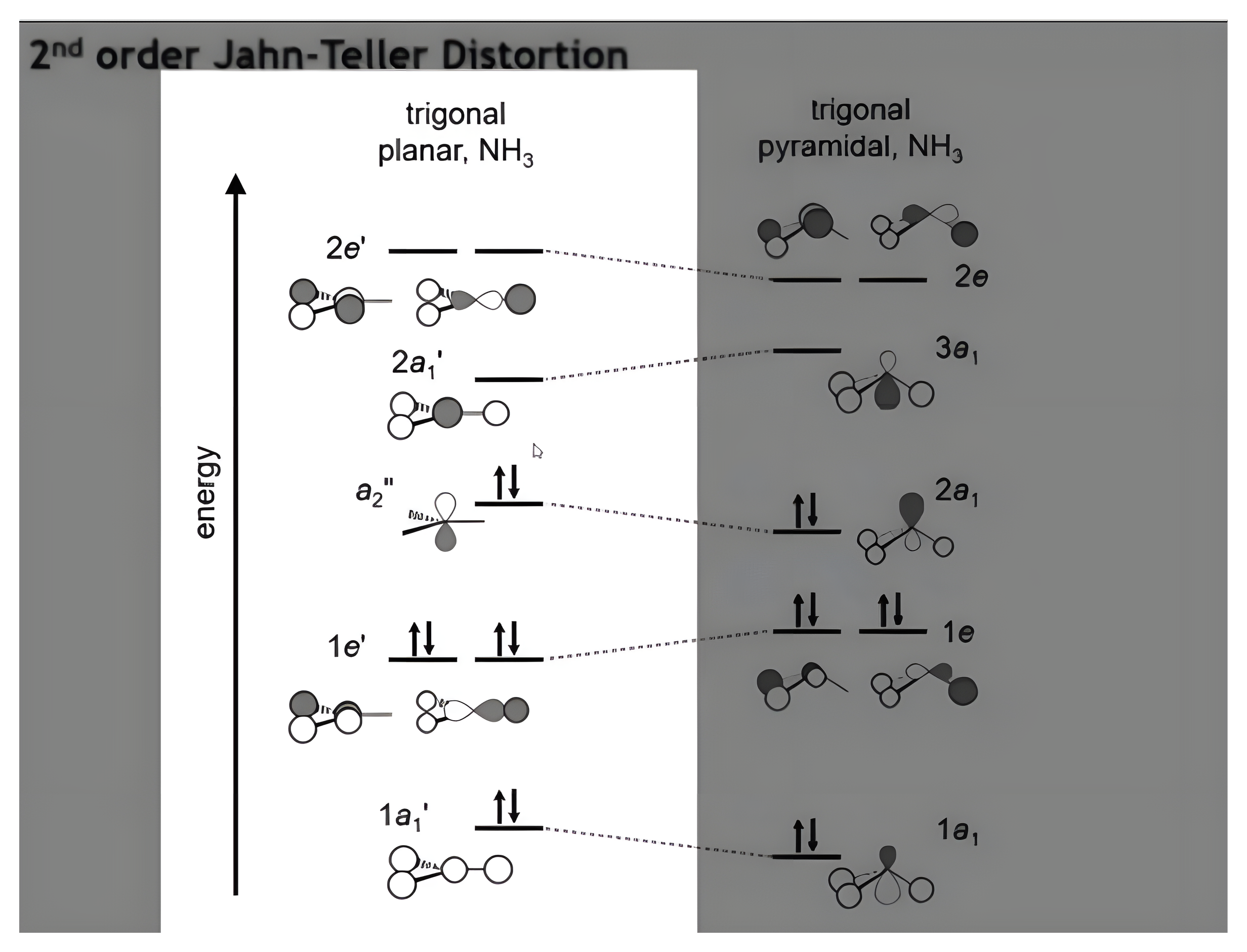
Second-Order Jahn–Teller: NH₃

Molecular-orbital correlation diagram for trigonal planar versus trigonal pyramidal ammonia, then the clean full diagram.

A second-order Jahn–Teller distortion is exemplified by ammonia (NH₃).

Hypothetical trigonal planar NH₃: 1A₁′ bonding N(2s)–H(1s), 2A₁′ its antibonding counterpart
1E′ bonding N(2pₓ, 2p_y)–H(1s), 2E′ antibonding counterpart
A₂″: nonbonding N(2p_z), cannot mix with H orbitals, serves as the HOMO
This configuration sets up a distortion that mixes the filled nonbonding orbital with nearby empty orbitals

[advance: bring up the full molecular-orbital diagram]

Ammonia is trigonal pyramidal, not planar, due to a second-order Jahn–Teller distortion
Planar → pyramidal: p_z and s both gain A₁ symmetry, allowing mixing between the HOMO (nonbonding p_z) and LUMO (antibonding 2s)
Result: a filled orbital mostly nonbonding but slightly bonding, and an empty orbital strongly antibonding
The filled orbital gains stability: density shifts toward the pyramid apex, a weakly bonding region; the antibonding orbital rises, but it’s unoccupied — no penalty
Occurs when the HOMO–LUMO gap is small and symmetry lowering enables mixing

The same second-order mixing shows up in the solid state with lead.

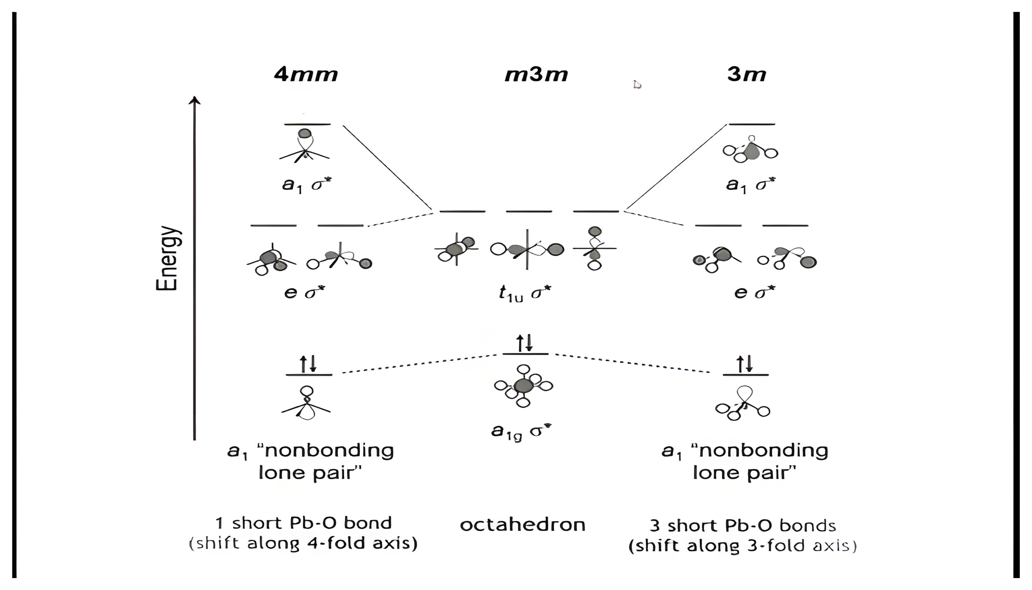
Pb²⁺ in an Octahedral Field

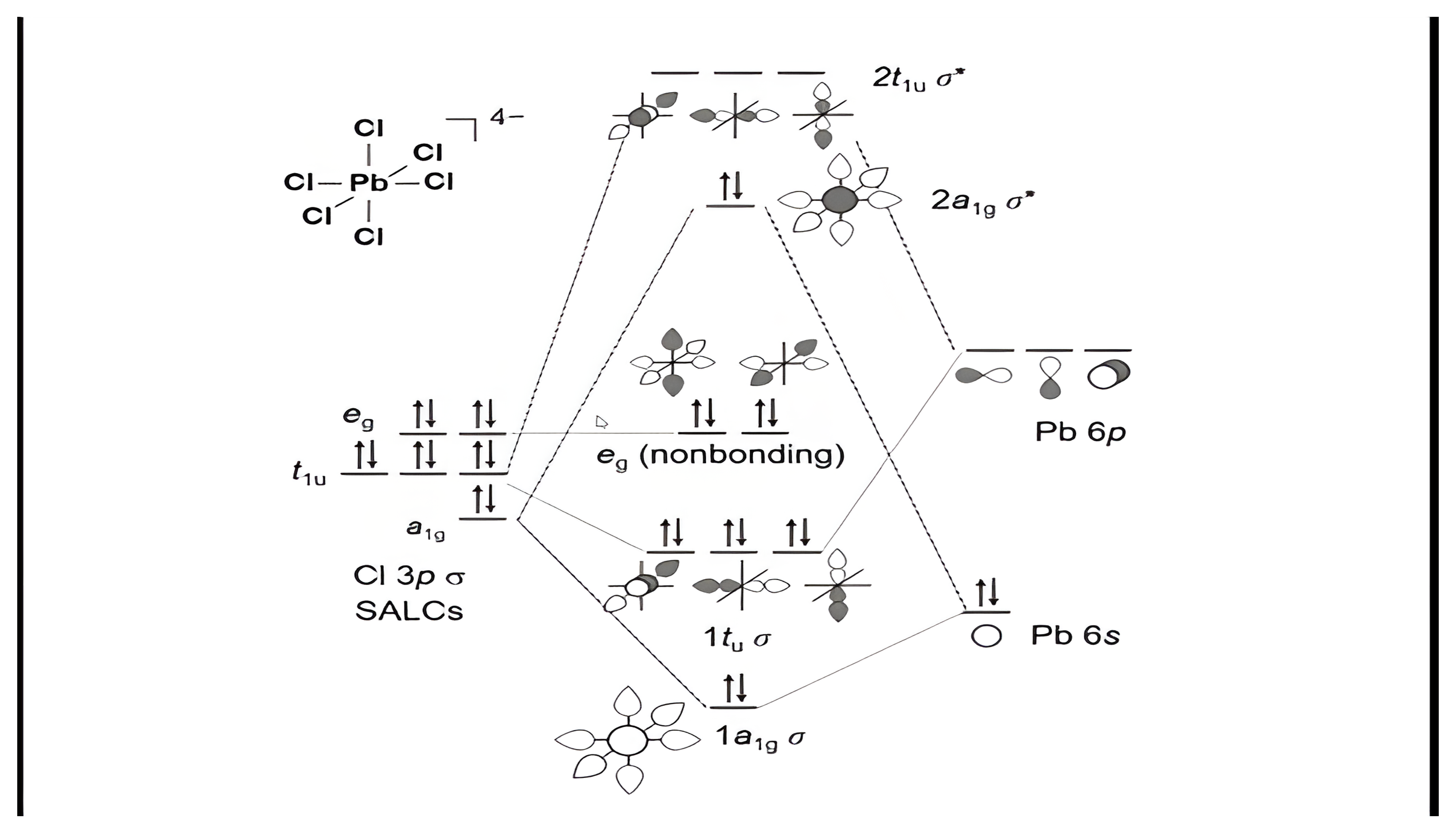
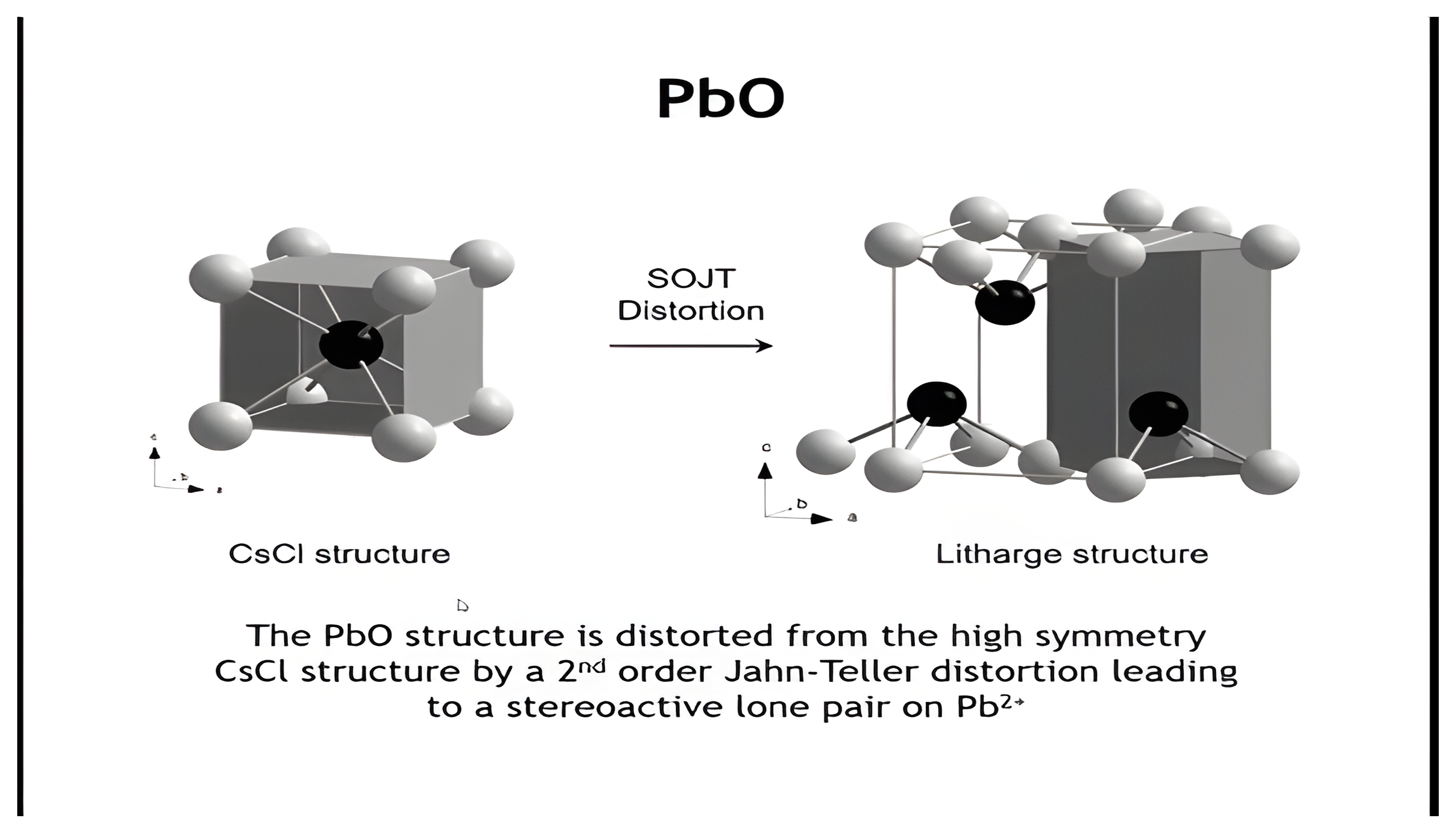
Molecular-orbital diagram of the PbCl6 4- octahedron built from lead 6s and 6p orbitals and chlorine 3p SALCs.

The Stereoactive Lone Pair

Energy diagram comparing the octahedral m3m geometry with distortions along the fourfold 4mm and threefold 3m axes that create the stereoactive lone pair.

PbO: From CsCl to Litharge

PbO distorting from the CsCl structure to the litharge structure by a second-order Jahn-Teller distortion.

Summary: Spin States & Jahn–Teller

Spin States & Jahn–Teller Distortions

Spin States

Δ = crystal-field splitting; P = spin-pairing energy.
Low spin (Δ > P): electrons pair in T₂g.
High spin (Δ < P): electrons spread across all d orbitals.
Δ↑ for 4d/5d metals, short/covalent bonds, strong-field ligands (CO > NH₃ > H₂O > Cl⁻).
Tetrahedral fields ≈ ½ Δ_oh → almost always high spin.

Octahedral → Square Planar (d⁸)

Ni²⁺ (3d⁸): weak field → octahedral (high spin).
Pt²⁺ (5d⁸): strong field → square planar (low spin).
Large Δ stabilizes dz², empties dx²–y².

Octahedral → Square Planar (d⁸)

Ni²⁺ (3d⁸): weak field → octahedral (high spin).
Pt²⁺ (5d⁸): strong field → square planar (low spin).
Large Δ stabilizes dz², empties dx²–y².

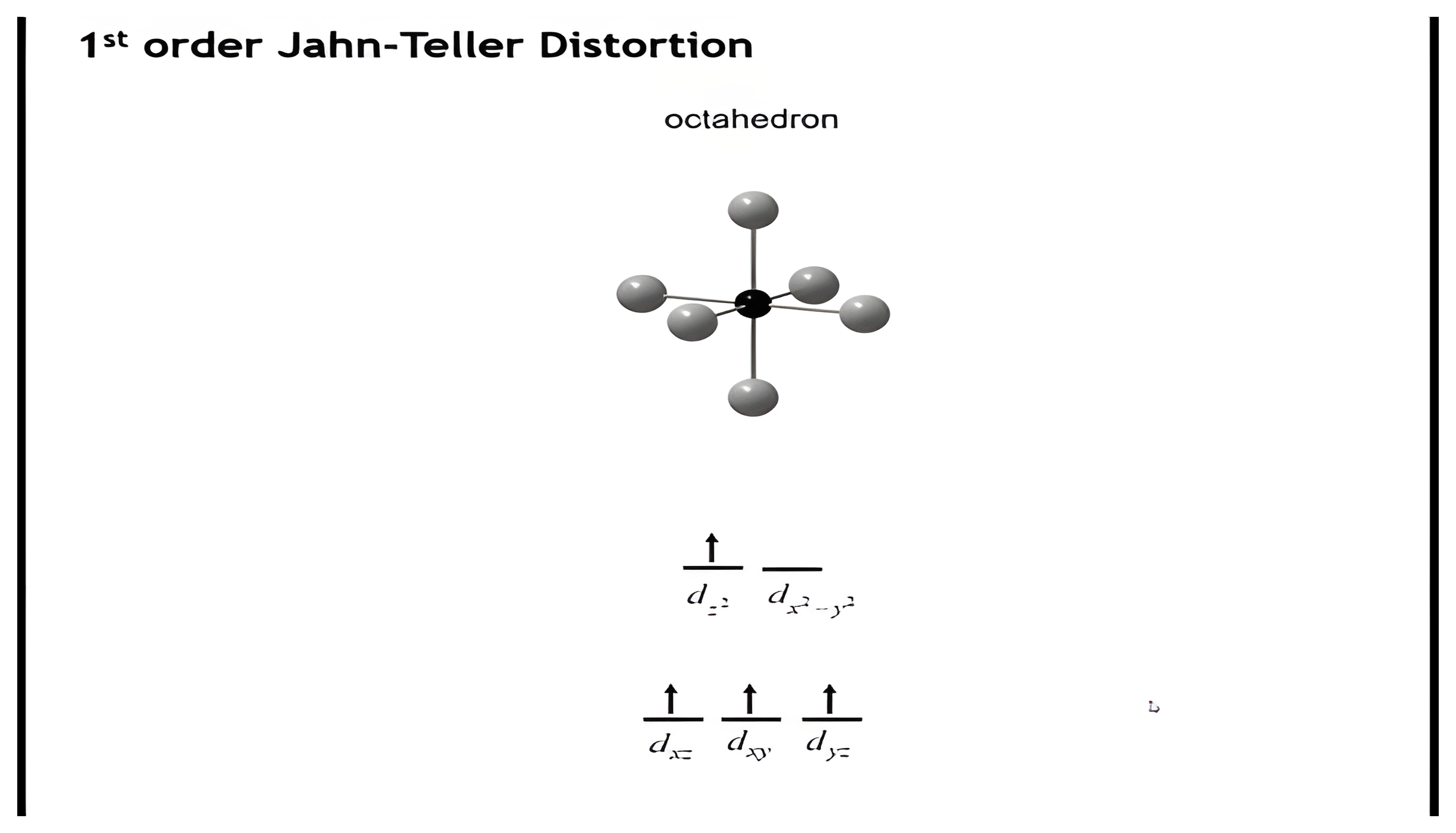
Jahn–Teller Distortion (1st Order)

Partially filled degenerate HOMO → symmetry lowering.
Seen in high-spin d⁴ (Mn³⁺) and d⁹ (Cu²⁺).
Elongated octahedra (4 short + 2 long bonds) most stable.
Compression rare.

2nd Order / Pseudo Jahn–Teller

Mixing between filled HOMO and nearby empty LUMO of same symmetry.
Examples:
- NH₃ – pz ↔ 2s mix → trigonal pyramidal.
- Pb²⁺, Sn²⁺ – 6s/6p mix → off-center “stereoactive lone pair.”
- d⁰ ions (Ti⁴⁺, Nb⁵⁺, Mo⁶⁺) – cation shifts off-center.

Core Idea: Electronic degeneracy and Δ vs P competition drive spin state and geometry distortions.

Okay, let’s summarize what we’ve seen.

Spin states: a balance of Δ and P — Δ large, pair up in the lower t₂g, low spin; Δ small, spread across all five d, high spin
Δ larger for 4d and 5d metals, short and more covalent bonds, strong-field ligands like CO and CN⁻; tetrahedral splitting about half → almost always high spin
d⁸: nickel, small Δ, stays octahedral; platinum, large Δ, distorts to square planar — dx²–y² pushed way up, the rest stabilized
Jahn–Teller: a partially filled degenerate orbital — high-spin d⁴ or d⁹ — distorts, usually elongating the octahedron, removing the degeneracy
Second-order: filled and empty orbitals of the same symmetry mix — why ammonia isn’t flat, why Pb²⁺ and Sn²⁺ shift off-center with a stereoactive lone pair, and the same in d⁰ oxides like Ti⁴⁺ or Nb⁵⁺
All from one principle: the system lowers its energy by changing how the d orbitals are occupied or mixed

To wrap up, test yourself on spin states.

Check Your Understanding: Spin States

Question 1 asking how the spin state of an Fe2+ d6 ion differs between the hexaaqua and hexacyanide complexes, then its answer.

Check Your Understanding: Jahn–Teller

Question 2 asking why Cu2+ d9 complexes show elongated rather than compressed octahedral geometry, then its answer.

Practice questions

Work the Lecture 13 practice questions before the next class. They cover molecular orbital theory, SALCs and frontier orbitals, MO diagrams for octahedral and tetrahedral complexes, spin states, and Jahn–Teller distortions.

Open the Lecture 13 practice questions

Every question carries a worked explanation, so you can check your reasoning as you go.

CHEM 548: Materials Chemistry

Lecture 13: Molecular Orbital Theory, Spin States, and Jahn–Teller Distortions

Learning Objectives: Molecular Orbital Theory

Molecular Orbitals

MO Diagram: H₂

Molecular Orbital Wavefunctions

MO Diagram: HHe

MO Diagram: O₂ and s–p Mixing

Beyond Diatomics: SALCs

BeH₂: MO Diagram and Frontier Orbitals

CH₄: MO Diagram

Delocalized $\pi$ Bonding in Benzene

Summary — Molecular Orbital Theory

Check Your Understanding: $\sigma$–$\pi$ Splitting

Check Your Understanding: SALCs

Learning Objectives: MO Theory Part II

Octahedral Complex: CrCl₆³⁻

Electron Counting: CrCl₆³⁻

CrCl₆³⁻: Bonding and Antibonding MOs

CrCl₆³⁻: Nonbonding MOs

CrCl₆³⁻: The Full MO Diagram

Tetrahedral Complex: CoCl₄²⁻

Electron Counting: CoCl₄²⁻

CH₄ Revisited

The t₂ and e Orbitals in a Tetrahedron

CoCl₄²⁻: The Full MO Diagram

Summary — MO Theory in Transition-Metal Complexes

Check Your Understanding: Field Splitting

Spin States & Jahn–Teller Distortions

Low-Spin and High-Spin Configurations

High spin vs. Low spin

Crystal Chemistry of Group 10 Monoxides

Octahedral vs. Square Planar

Jahn–Teller Distortions

First-Order Jahn–Teller Distortion

Distortions in d⁹ and d¹⁰ Halides

Jahn–Teller Distortions: s–dz² Mixing

Second-Order Jahn–Teller: NH₃

Pb²⁺ in an Octahedral Field

The Stereoactive Lone Pair

PbO: From CsCl to Litharge

Summary: Spin States & Jahn–Teller

Check Your Understanding: Spin States

Check Your Understanding: Jahn–Teller

Practice questions

Jahn–Teller Distortions: s–d_z² Mixing