CHEM 548: Materials Chemistry
Lecture 11: Free Energy, Phase Diagrams, and Ionic Bonding
Reading: Woodward, Karen, Evans, and Vogt, Solid State Materials Chemistry
Ch. 5, §5.1
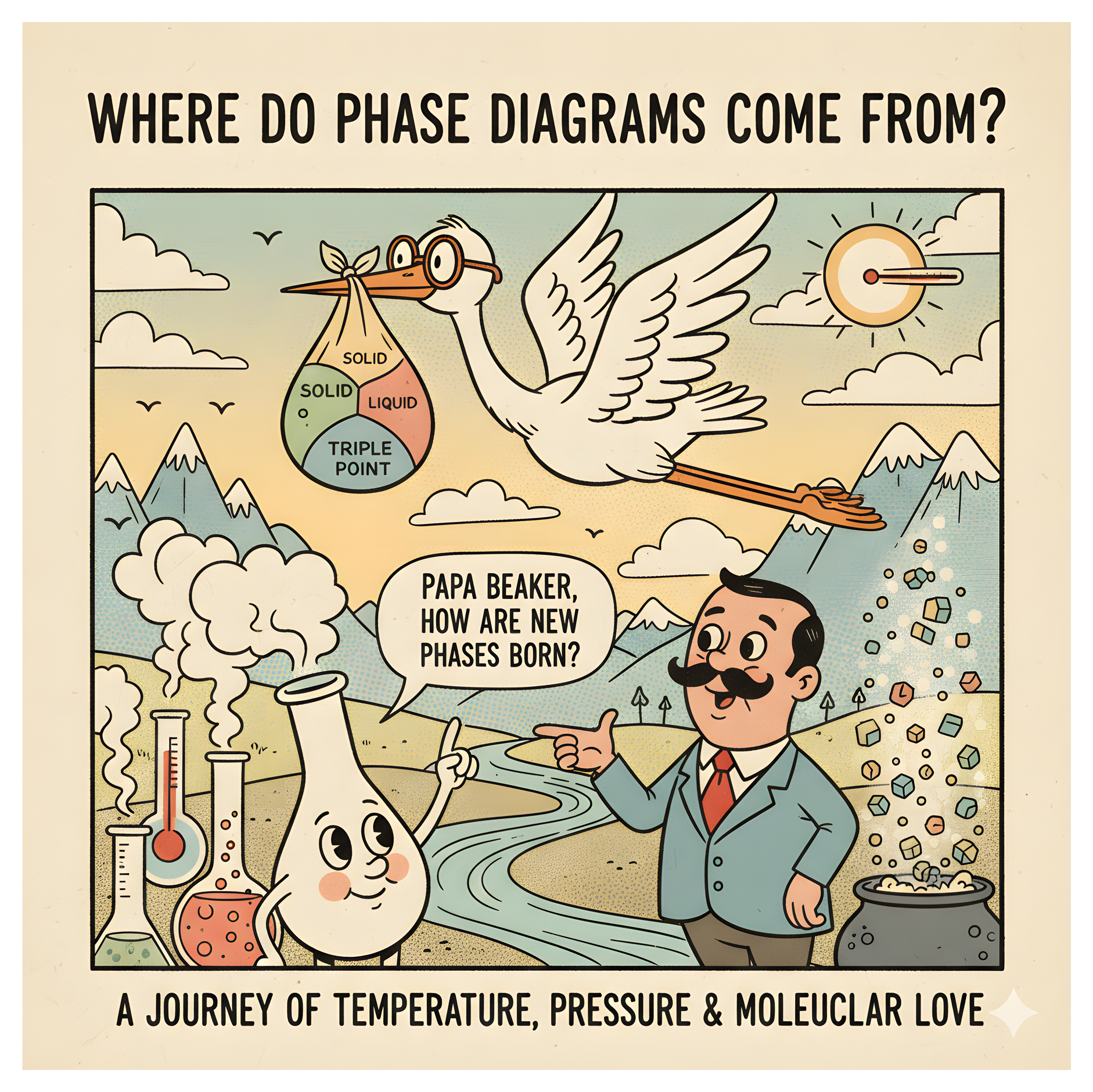
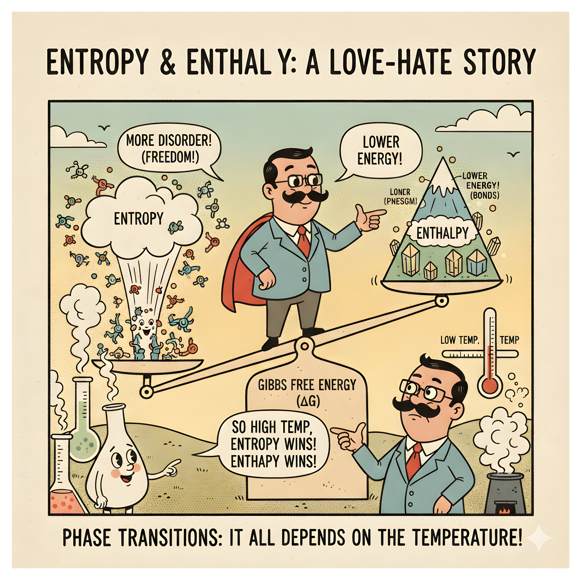
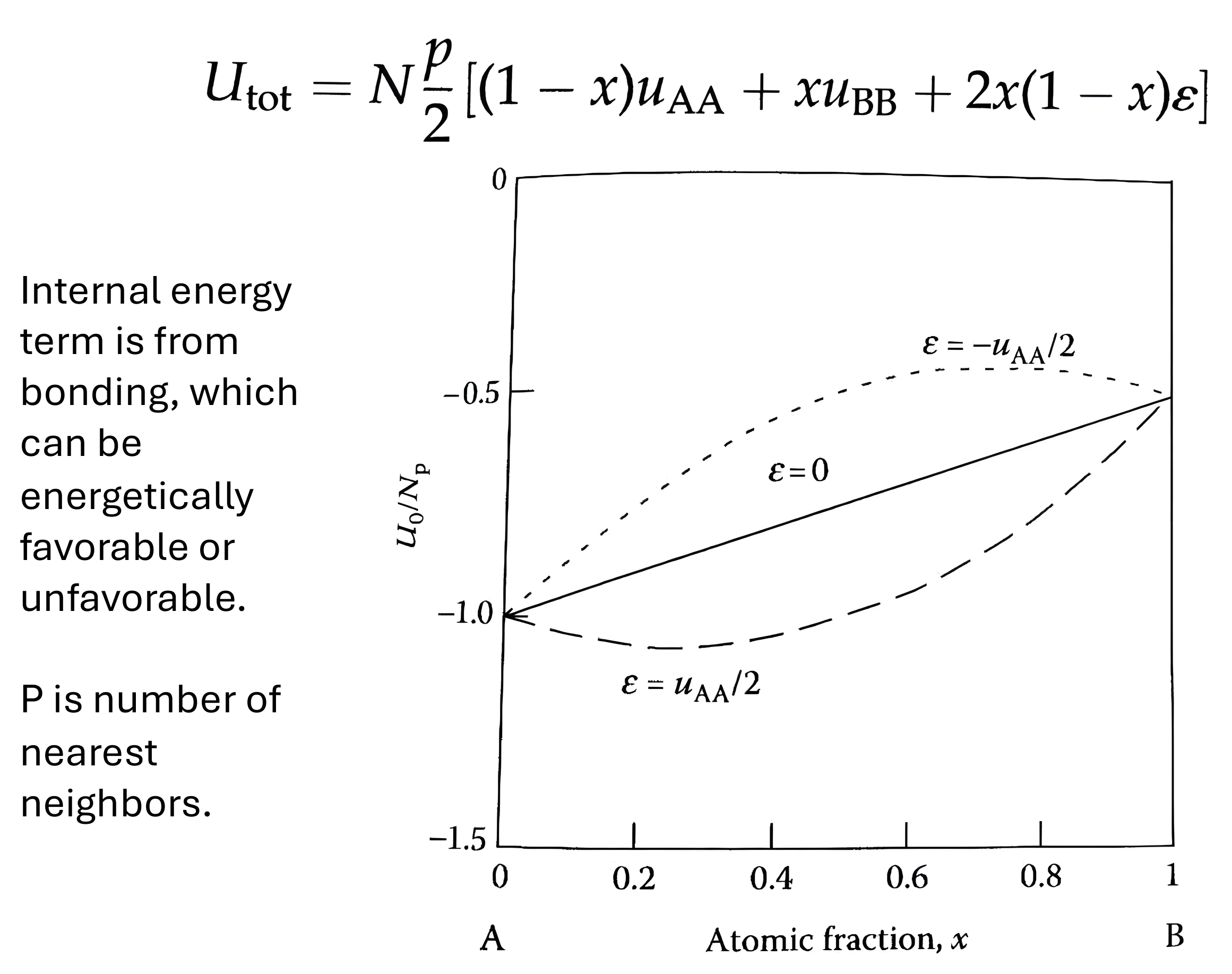
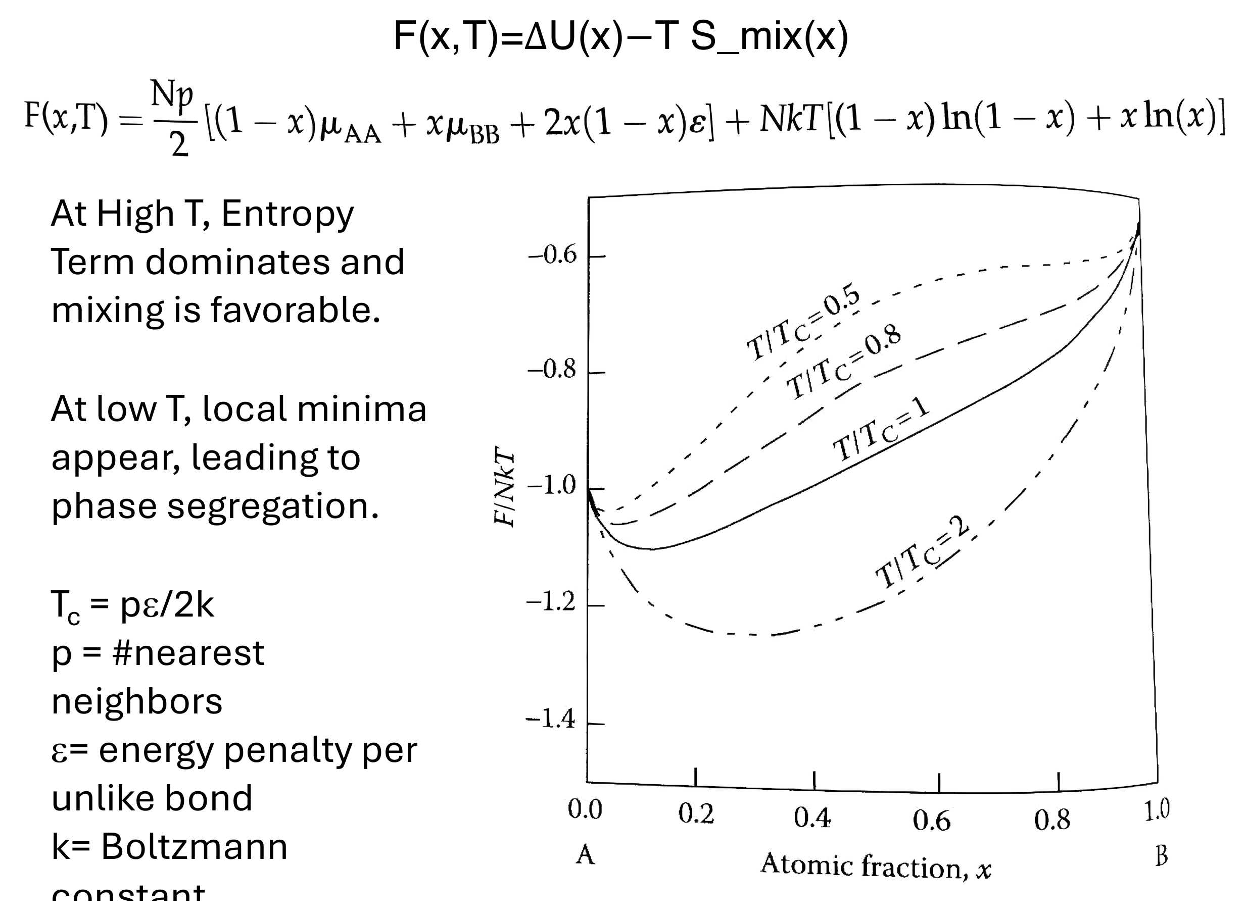
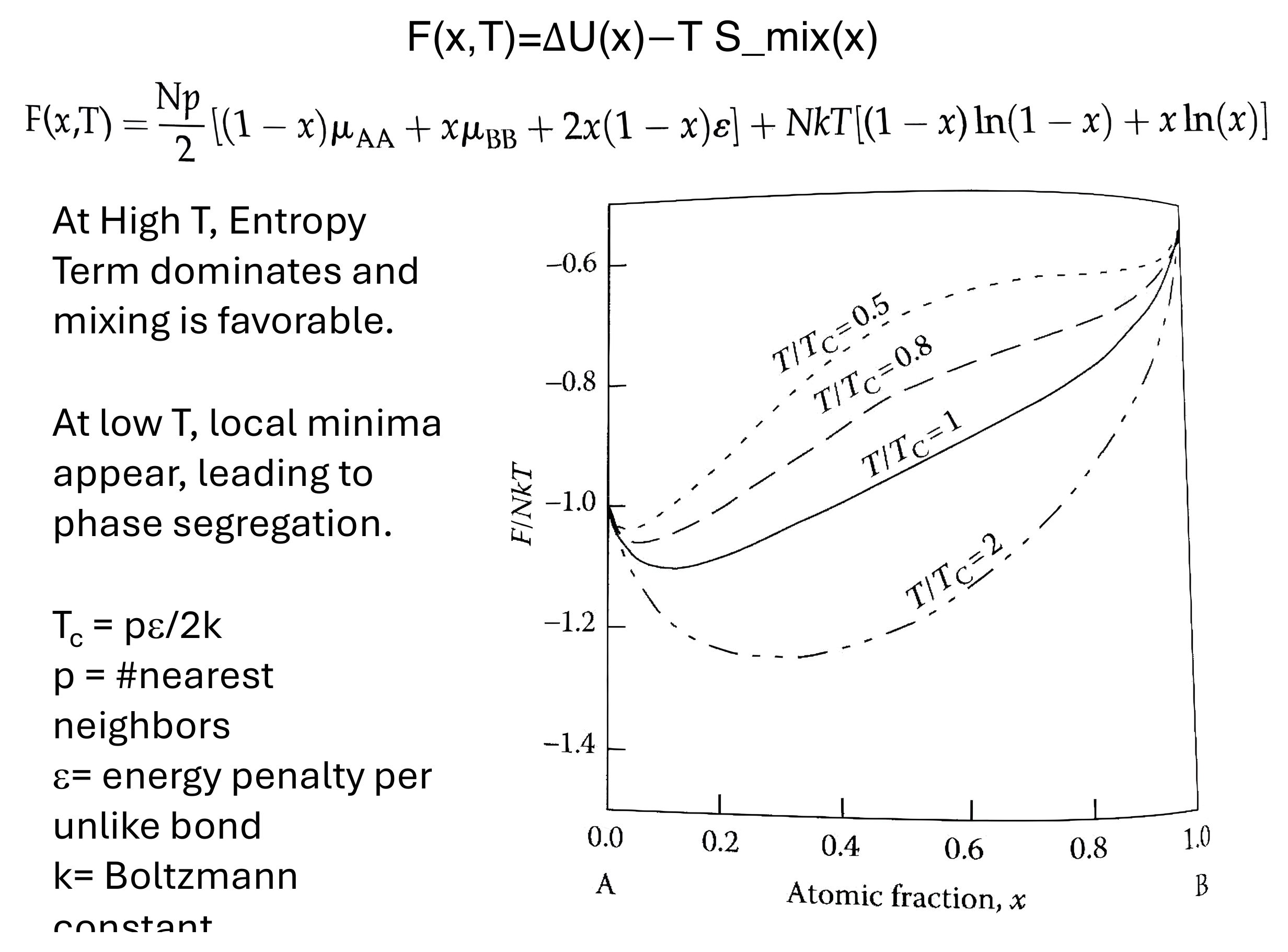
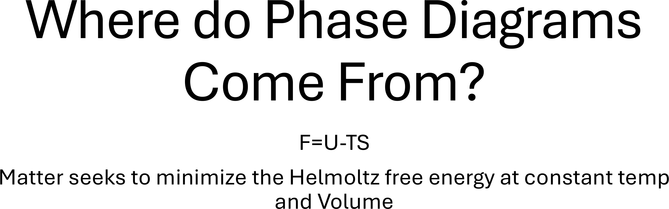 $F=U-TS$
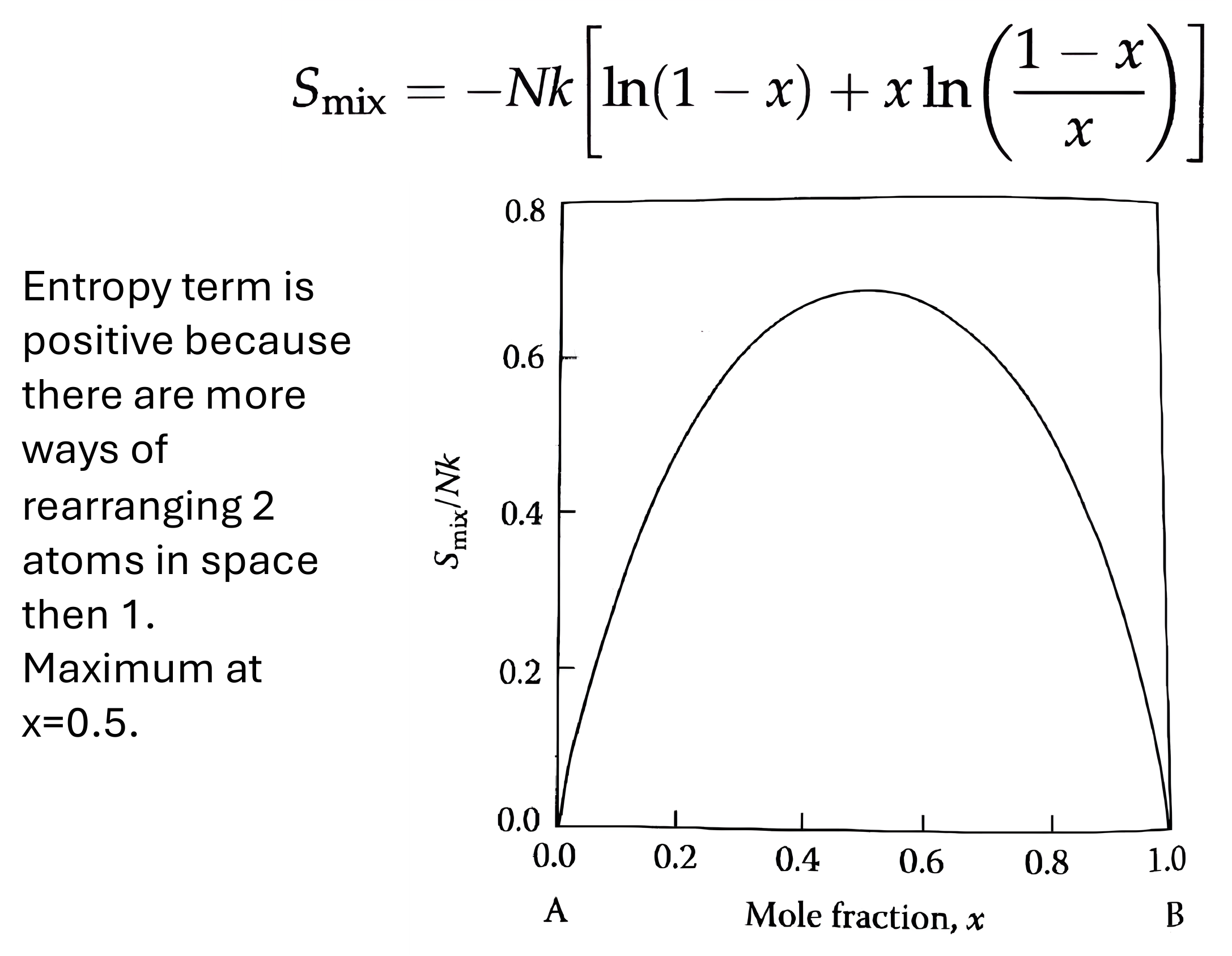
Homework Questions
- Define the parameter ε in the mean-field model of mixing. Physically, what does it mean if ε < 0? What about ε > 0?
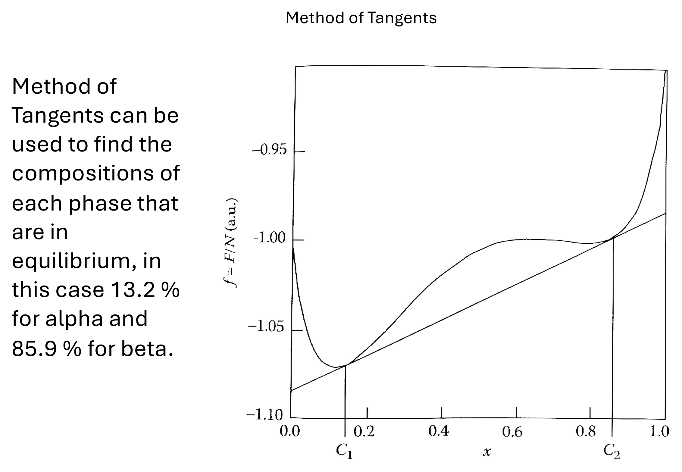
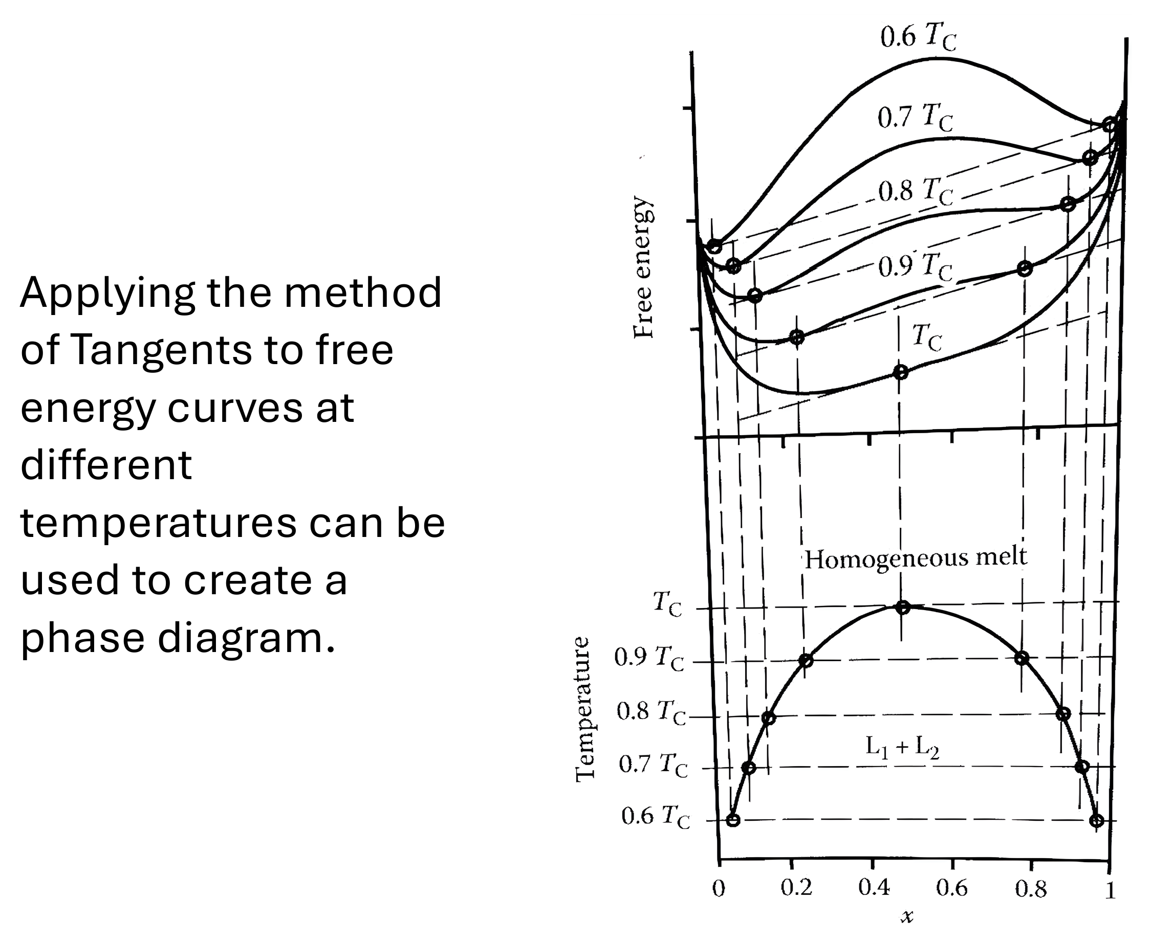
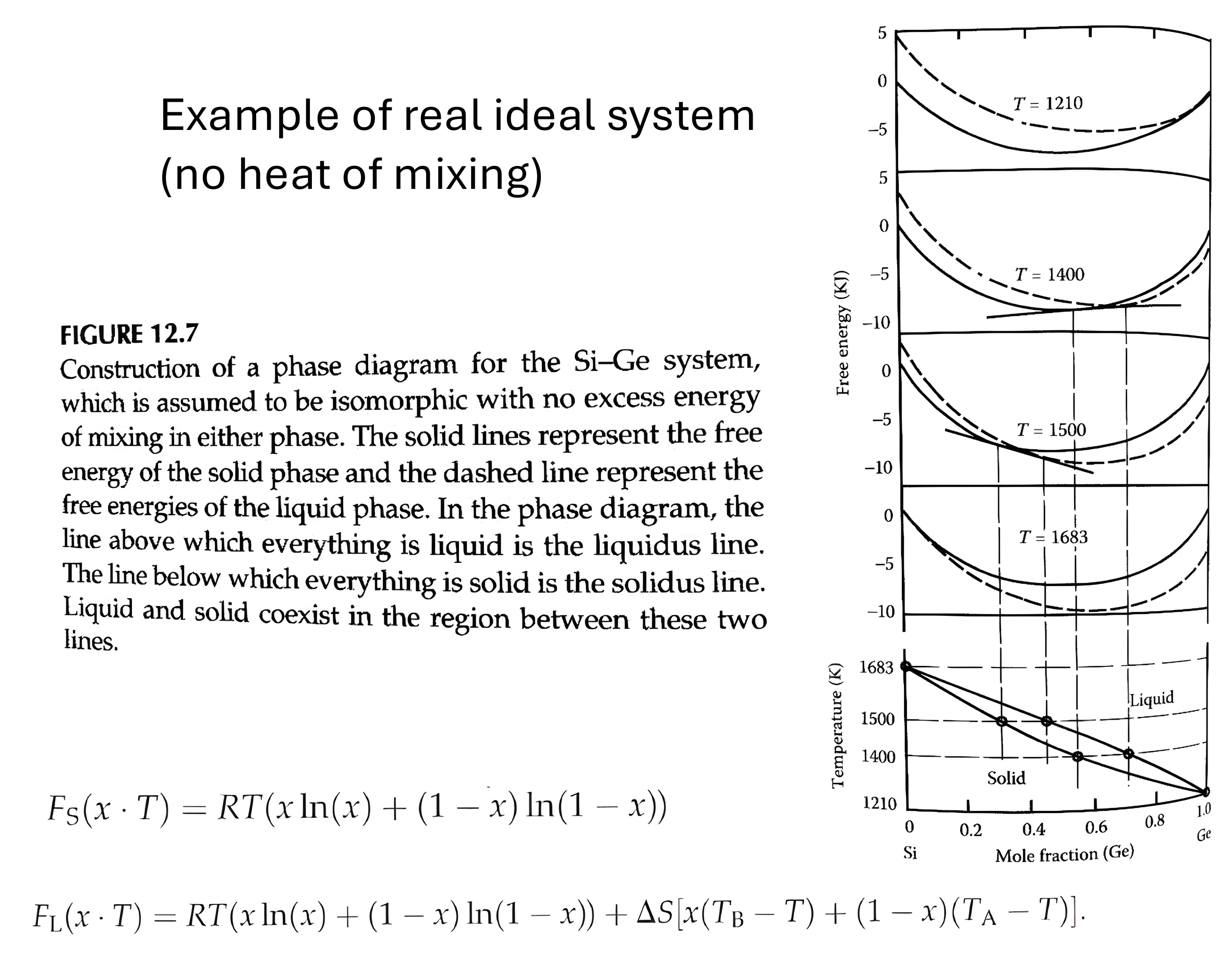
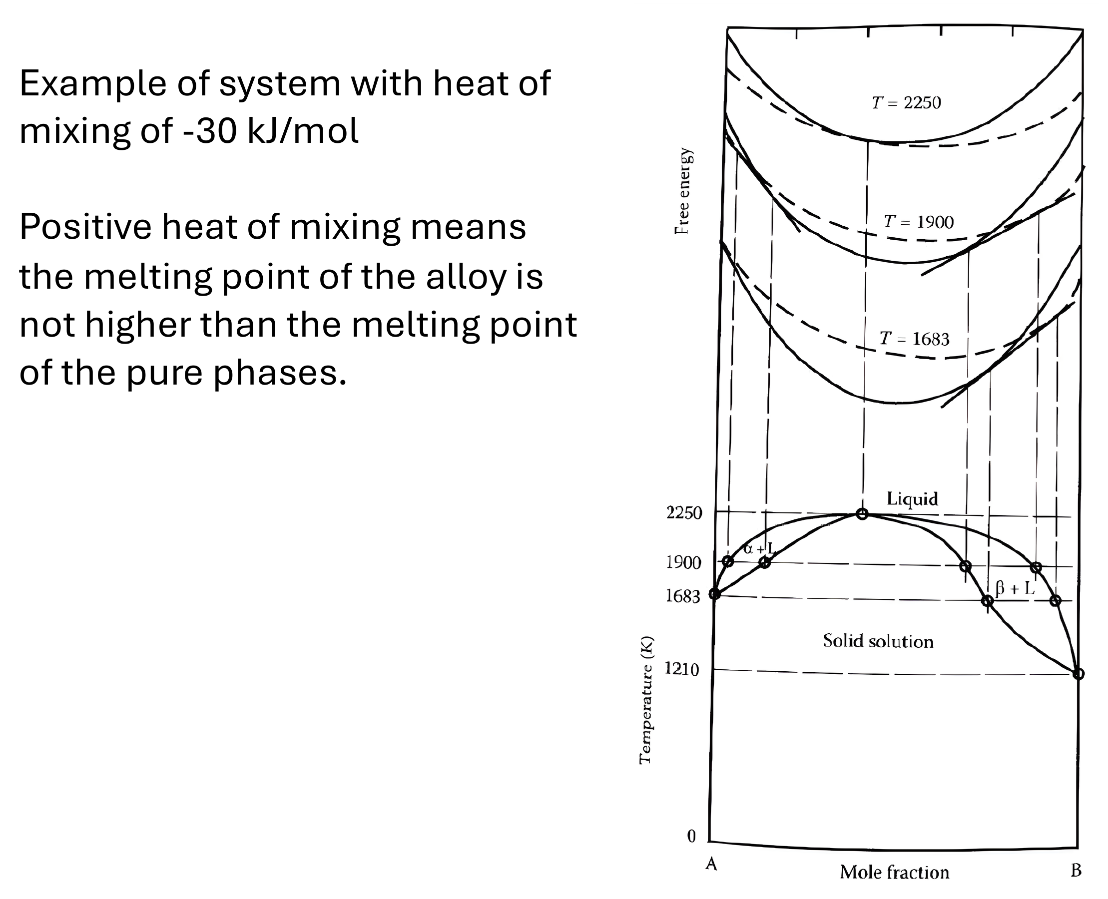
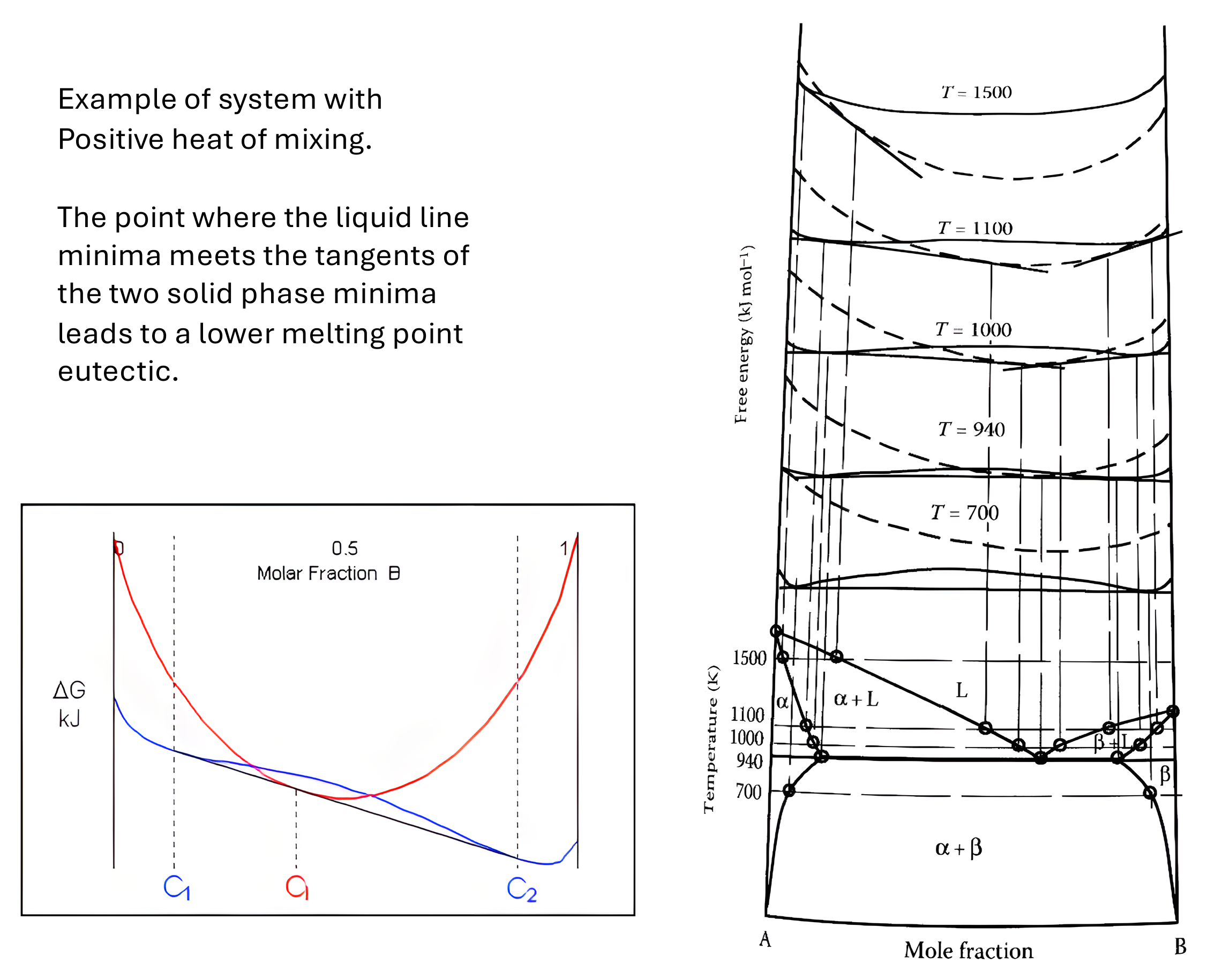
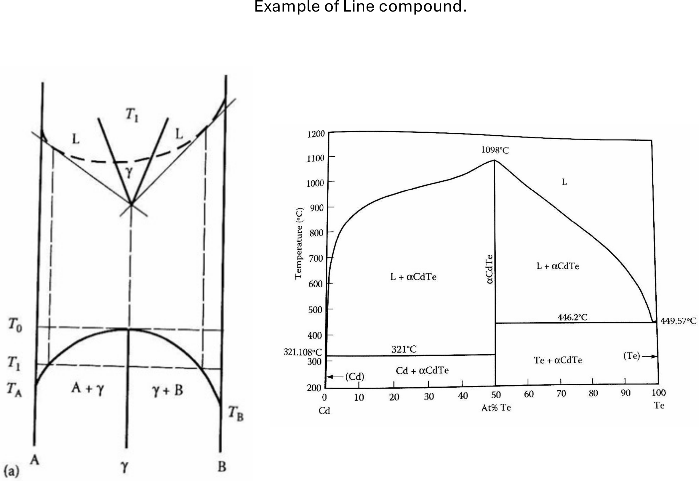
- Contrast the phase diagram topologies of an isomorphous alloy (Si–Ge) and an endothermically mixing alloy (with a eutectic). What underlying free-energy features produce the differences?
- Calculate the entropy of mixing (per mole, in J/mol·K) for a binary solution with mole fraction xA = 0.25, xB = 0.75. Use R = 8.314 J/molK.
- Using the regular solution model with p = 12, ε = 12 meV, compute the critical temperature Tc. Express your answer in Kelvin.
(Constants: 1 eV = 1.602 × 10⁻¹⁹ J, kB = 8.617 × 10⁻⁵ eV/K).
Ionic Bonding
By the end of this lecture, you should be able to:
- Explain why chemical bonding connects structure to properties of materials.
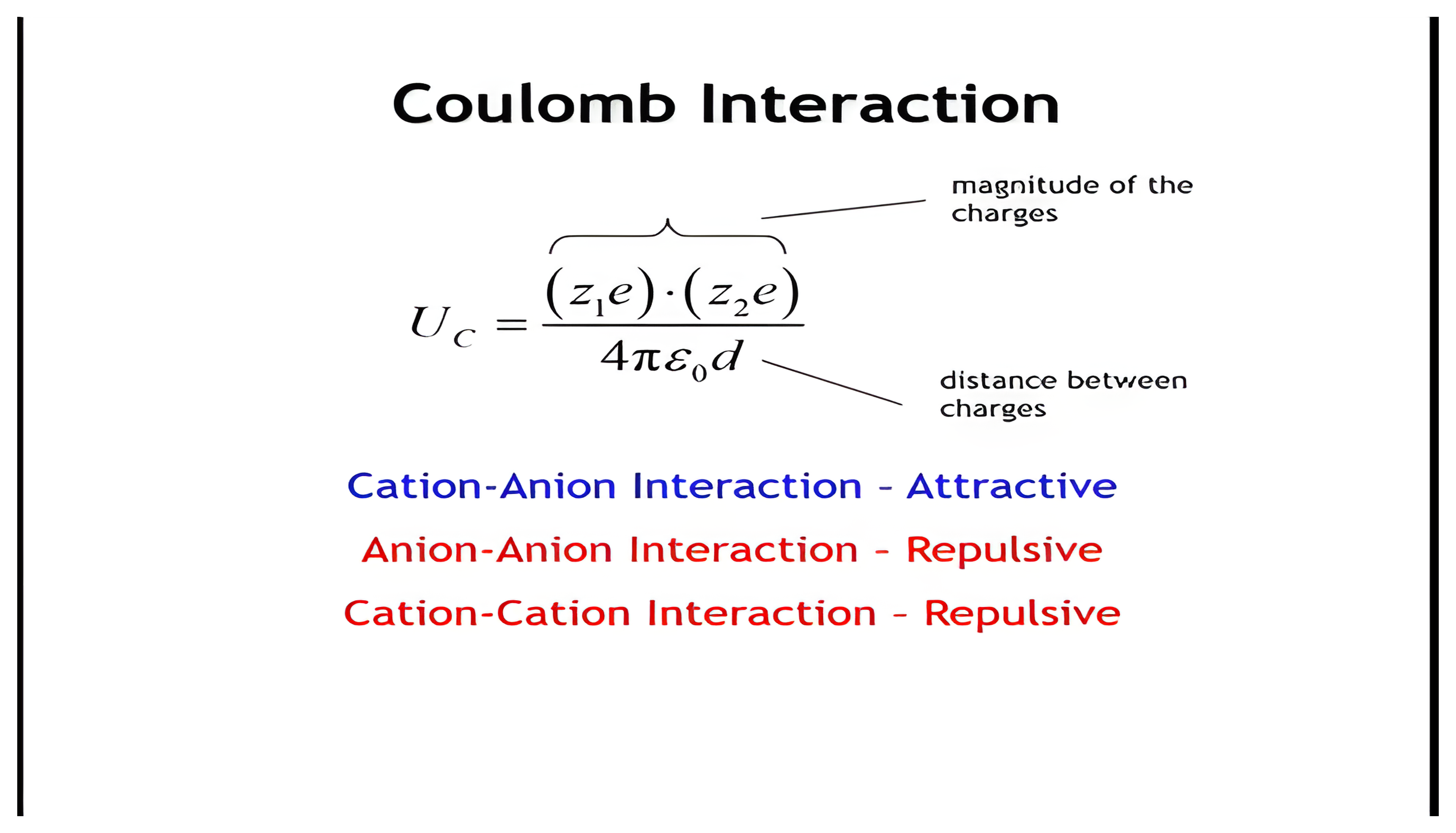
- Define ionic bonding as electrostatic interactions between point charges.
- Apply Coulomb’s law to estimate attractive vs. repulsive interactions between ions.
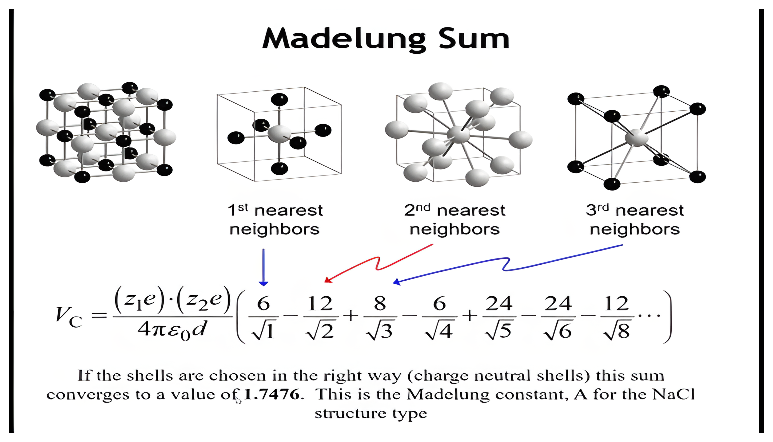
- Describe how coordination number and structure type affect the Madelung constant.
- Explain what the Madelung constant represents and why it differs for NaCl, CsCl, ZnS, etc.
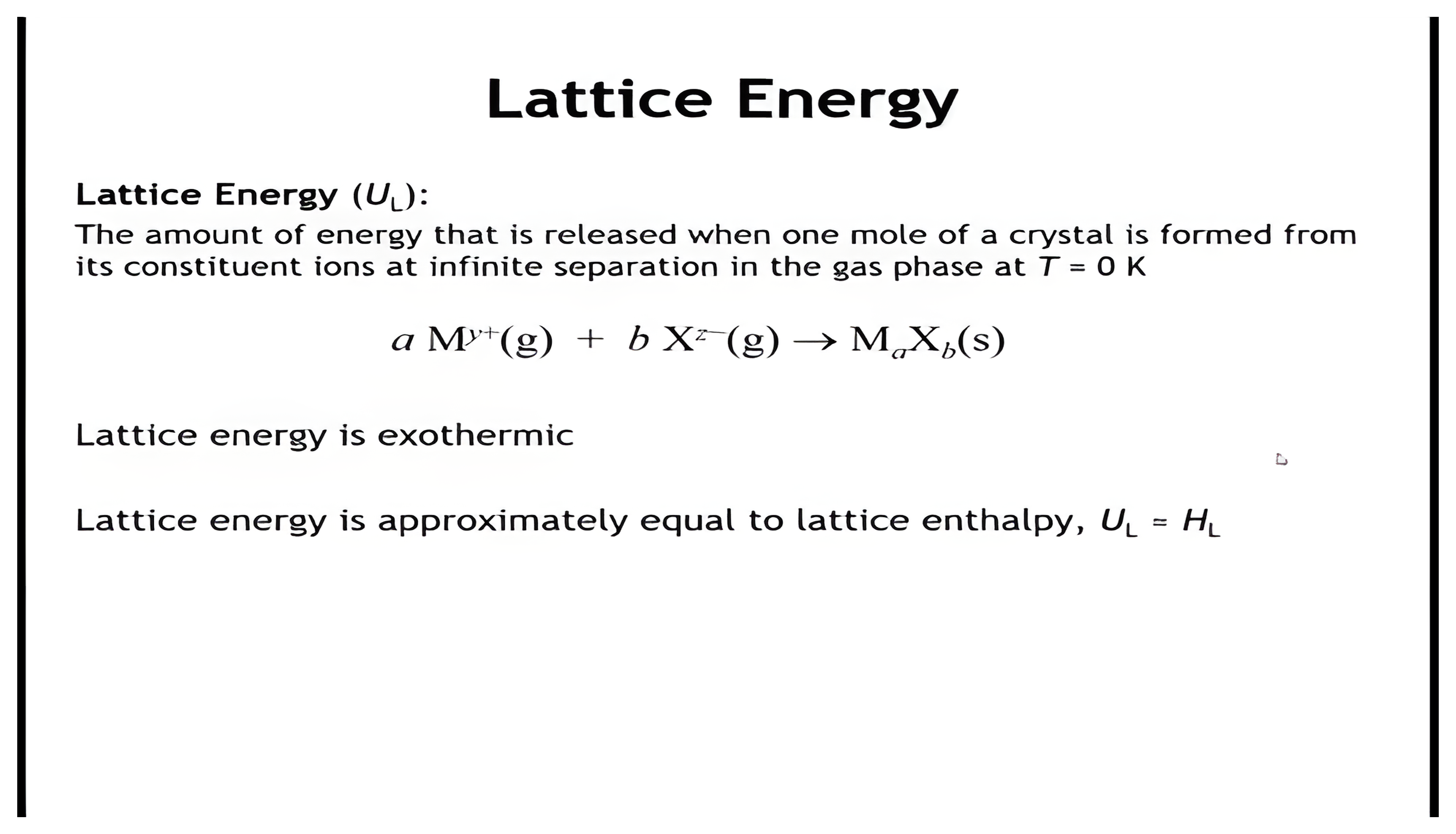
- Define lattice energy and distinguish between lattice energy and lattice enthalpy.
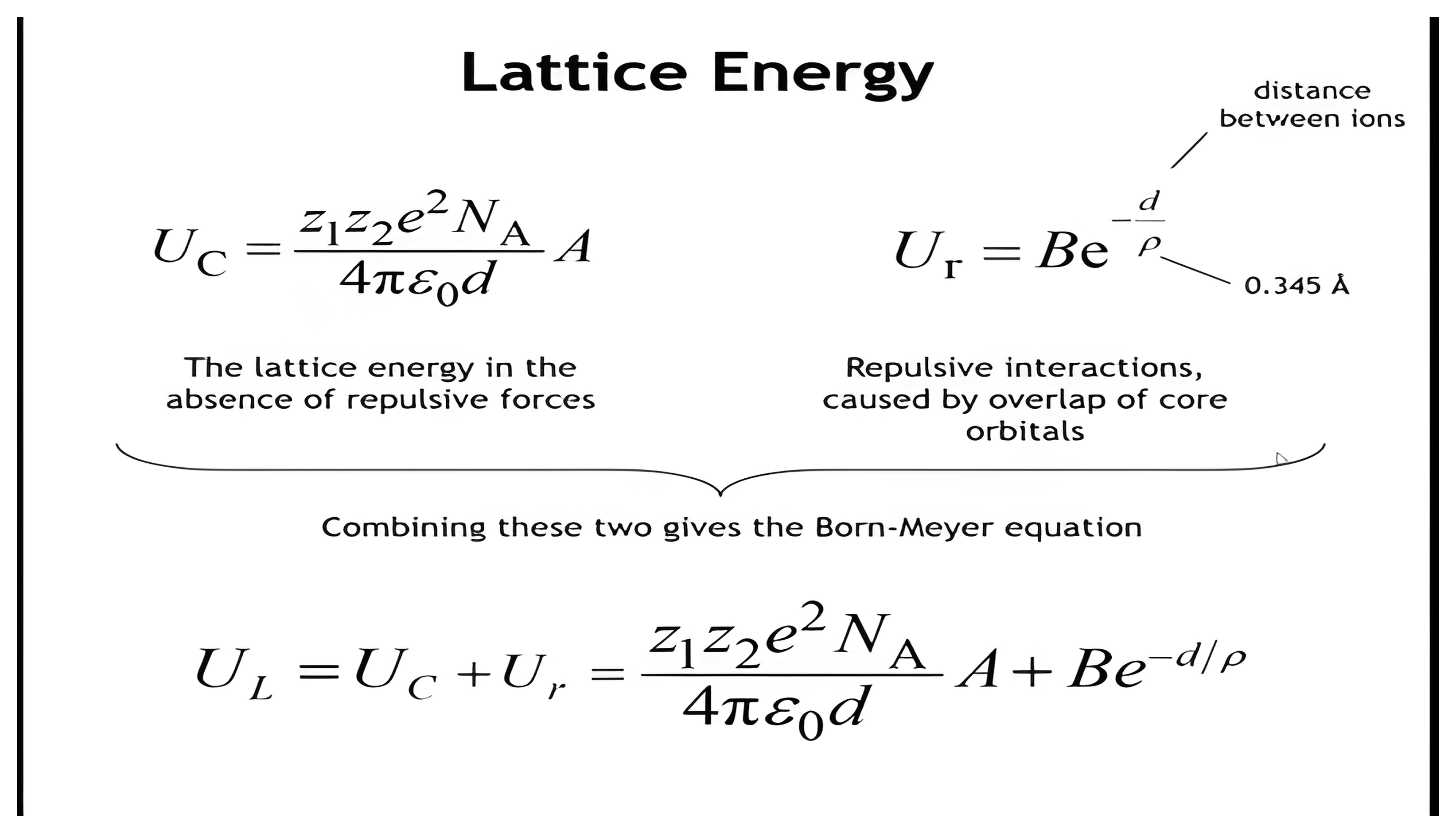
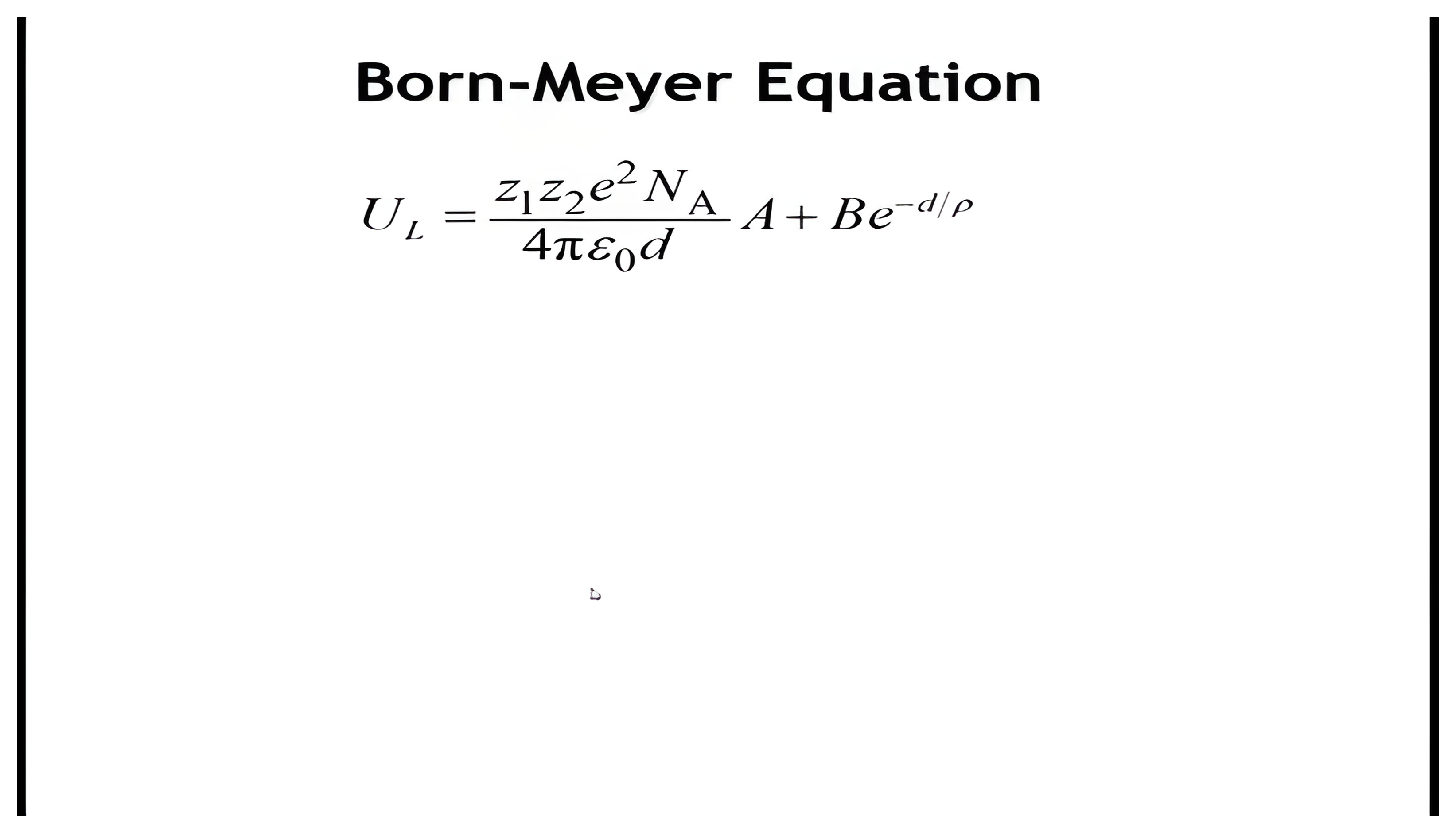
- Use the Born–Mayer equation to estimate lattice energies, recognizing the role of repulsive terms.
Madelung Constants and Structure Type
| Structure Type | Coordination | A | Structure Type | Coordination | A |
|---|---|---|---|---|---|
| Cesium chloride | Cs[8]Cl[8] | 1.763 | Fluorite | Ca[8]F₂[4] | 2.519 |
| Rock salt | Na[6]Cl[6] | 1.748 | Rutile | Ti[6]O₂[3] | 2.408 |
| Wurtzite | Zn[4]S[4] | 1.641 | Cadmium chloride | Cd[6]Cl₂[3] | 2.244 |
| Zinc blende | Zn[4]S[4] | 1.638 | Cadmium iodide | Cd[6]I₂[3] | 2.192 |
Electrostatic interactions favor symmetric structures with close packing of anions and cations and high coordination numbers.
Summary – Chapter 5: Ionic Bonding
- Bonding refresher bridges earlier crystal structure topics to upcoming band structure.
- Ionic bonding model: treat ions as point charges; interaction energy from Coulomb’s law.
- Attractive vs. repulsive forces depend on charge sign and distance.
- Long-range nature of Coulomb interactions requires summing over all shells of neighbors.
- Summation leads to the Madelung constant (e.g., 1.748 for NaCl rock salt).
- Higher coordination → larger Madelung constant → stronger bonding.
- Layered structures (e.g., CdCl₂, CdI₂) show reduced Madelung constants due to added cation–cation repulsions.
- Lattice energy = energy released when ions form a solid from infinite separation (exothermic).
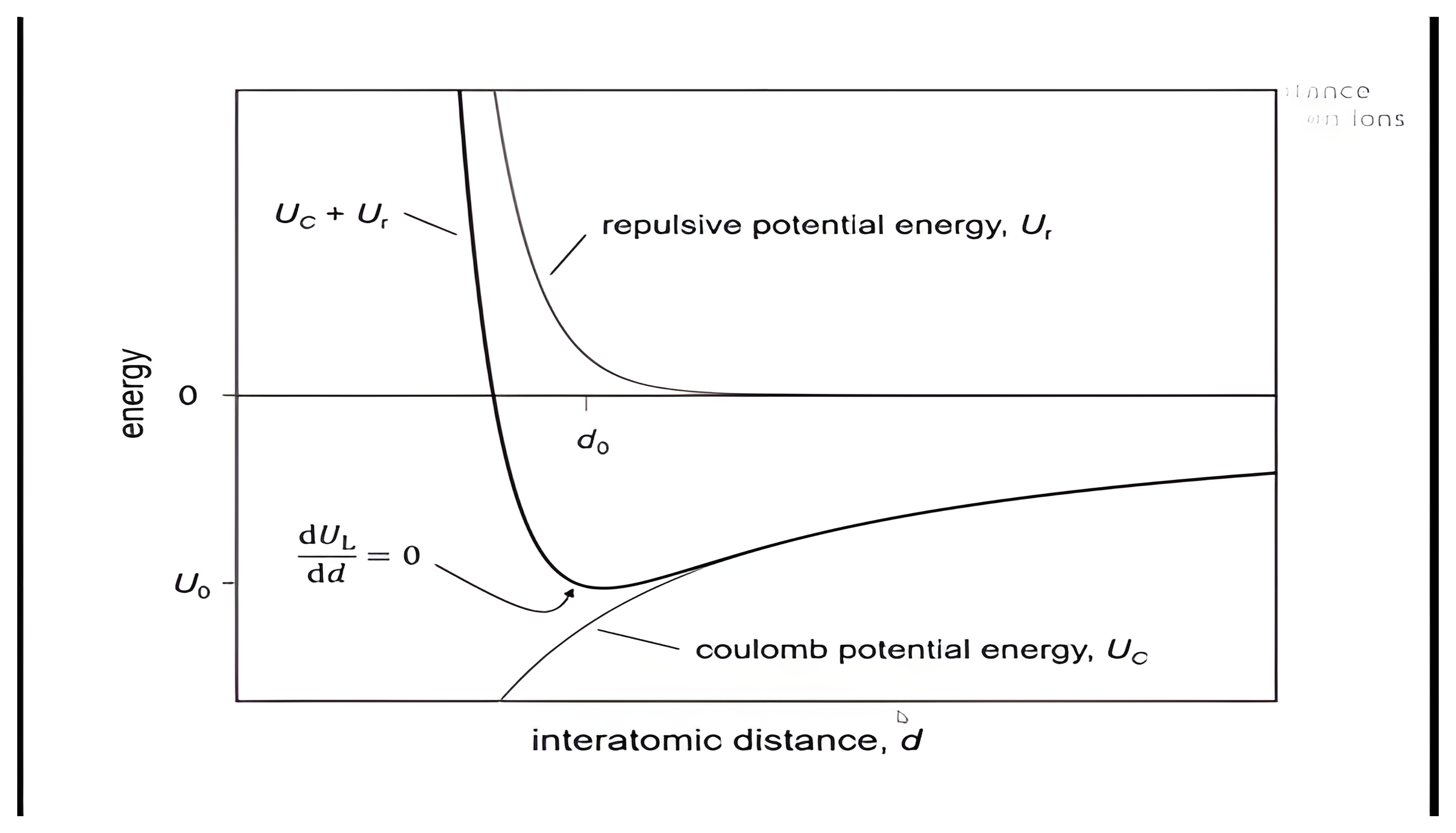
- Born–Mayer model combines:
- Coulombic attraction (favors collapse),
- Exponential repulsion (prevents collapse),
- Minimum → equilibrium distance d₀.
- Born–Mayer equation allows quantitative lattice energy estimates using charges, Madelung constant, and ionic radii.

Part 2
By the end of this lecture, you should be able to:
- Recall the form and physical meaning of the Born–Mayer equation.
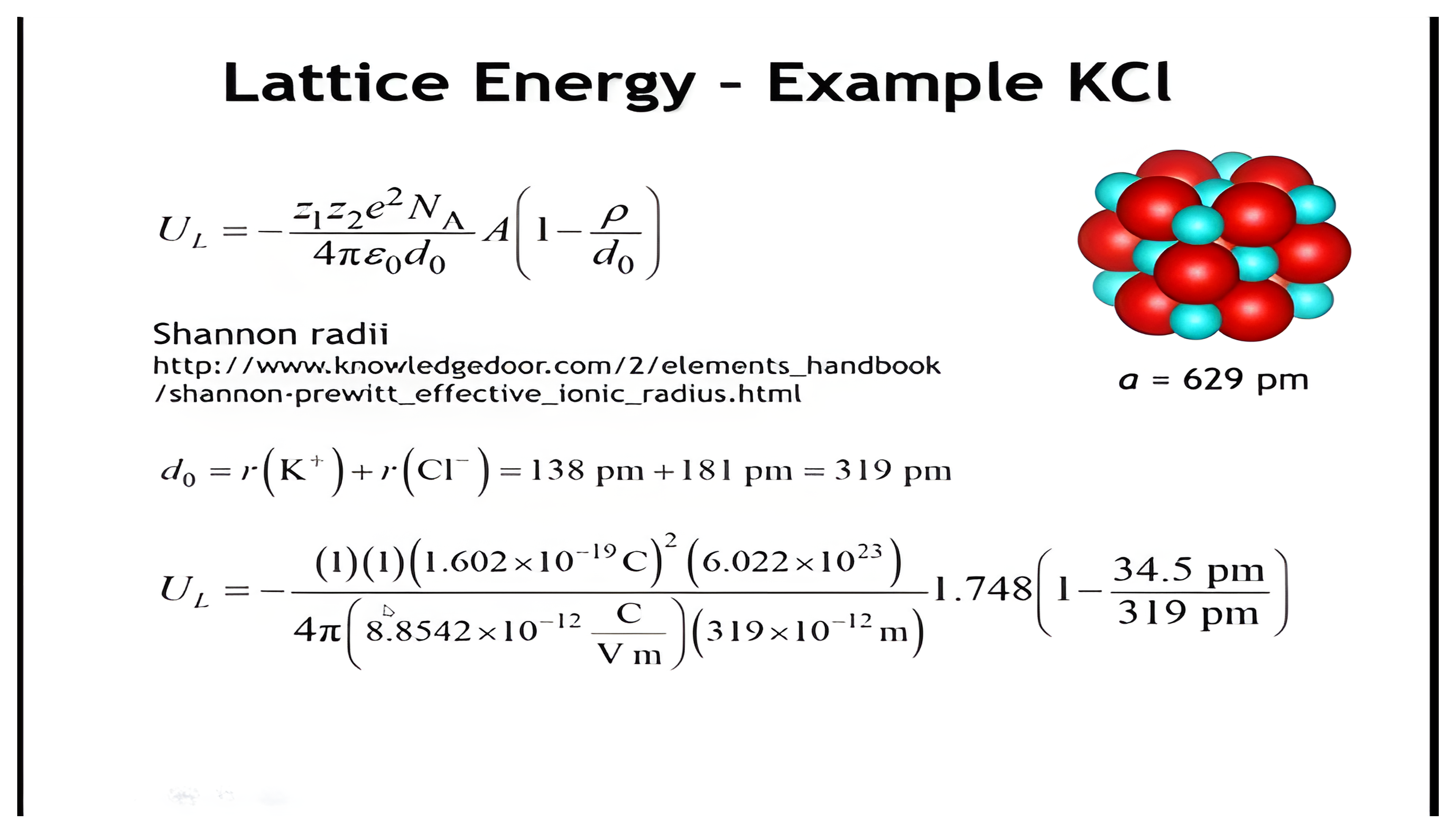
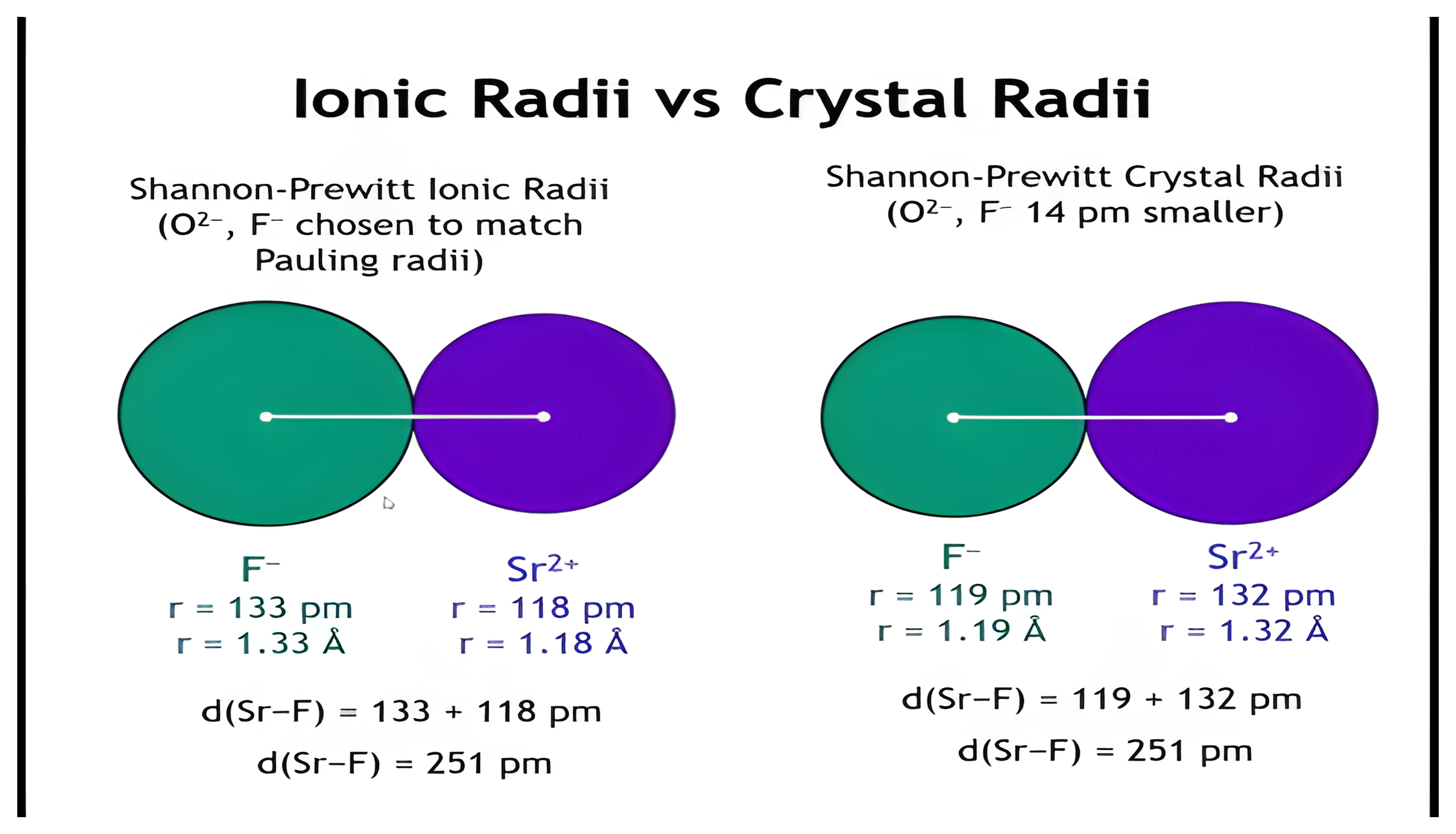
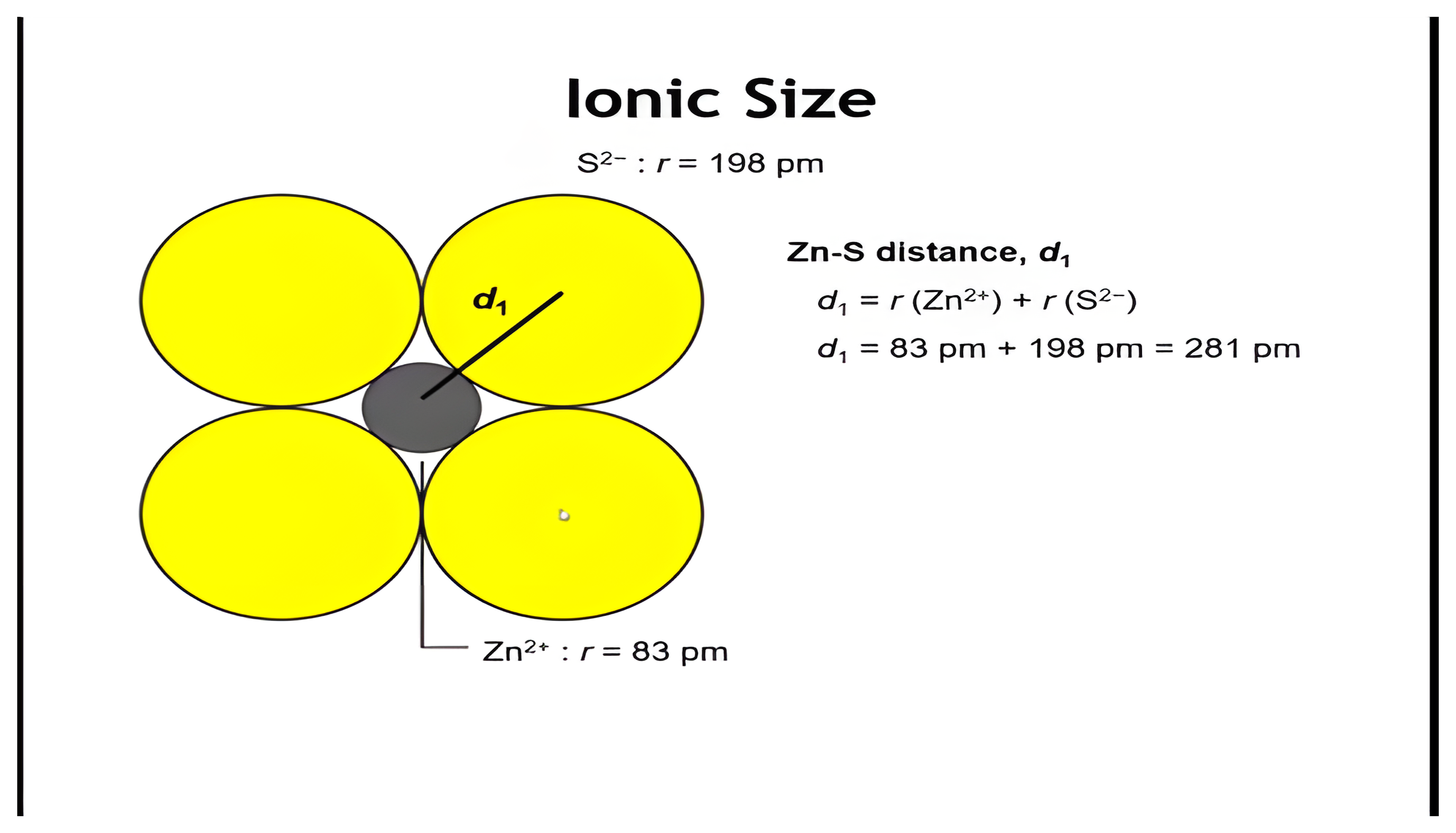
- Use ionic radii (Shannon radii) to estimate the equilibrium distance d₀.
- Calculate the lattice energy of an ionic compound (example: KCl, rock salt structure).
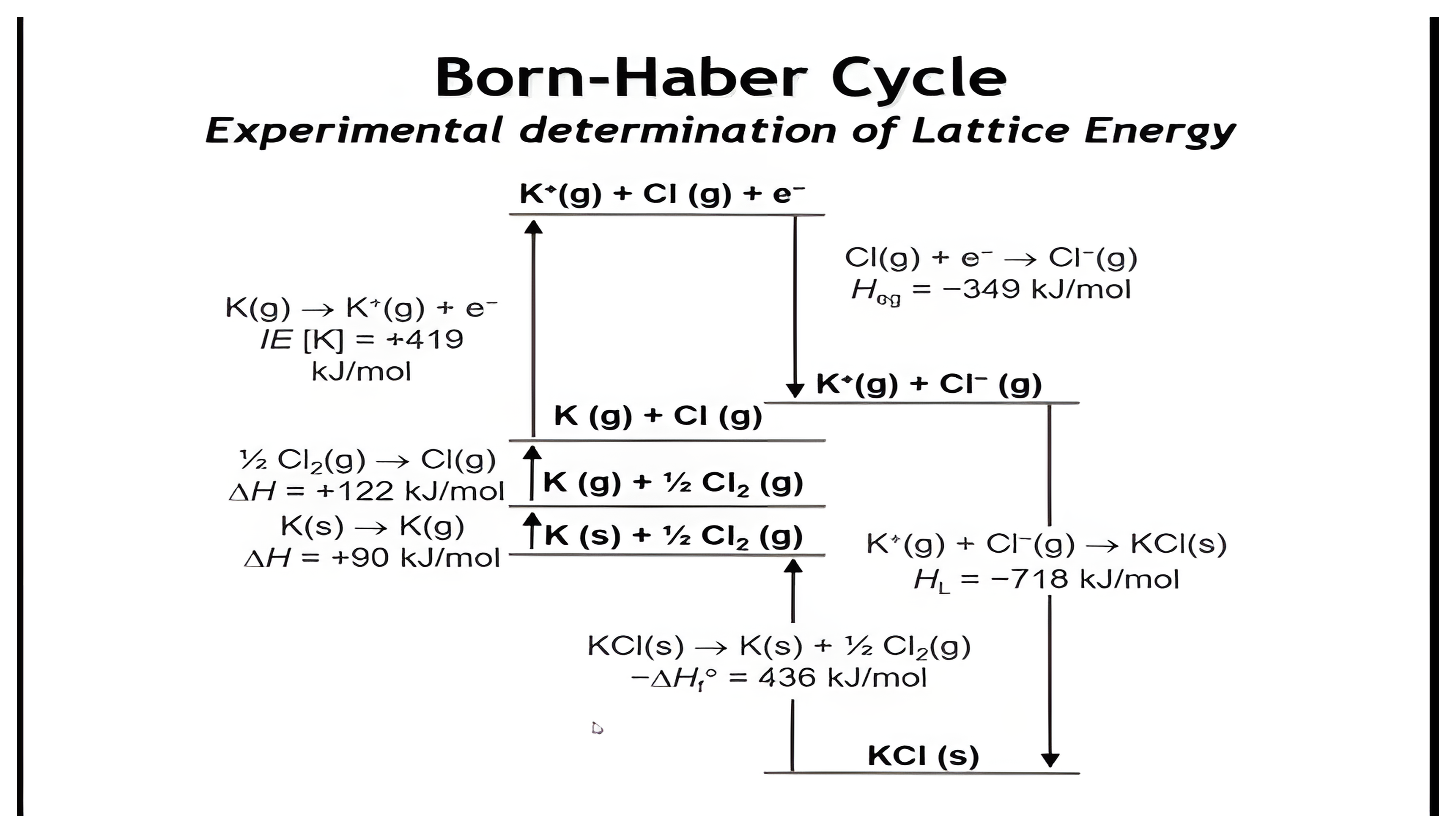
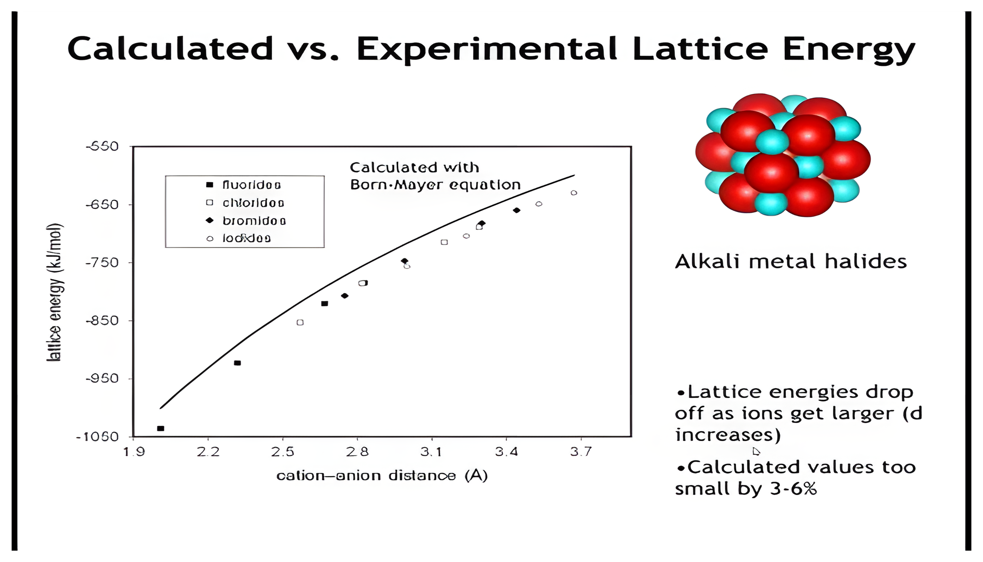
- Compare calculated lattice energies to experimental values obtained from the Born–Haber cycle.
- Explain why the Born–Mayer equation underestimates lattice energies and identify additional corrections (dispersion, zero-point energy).
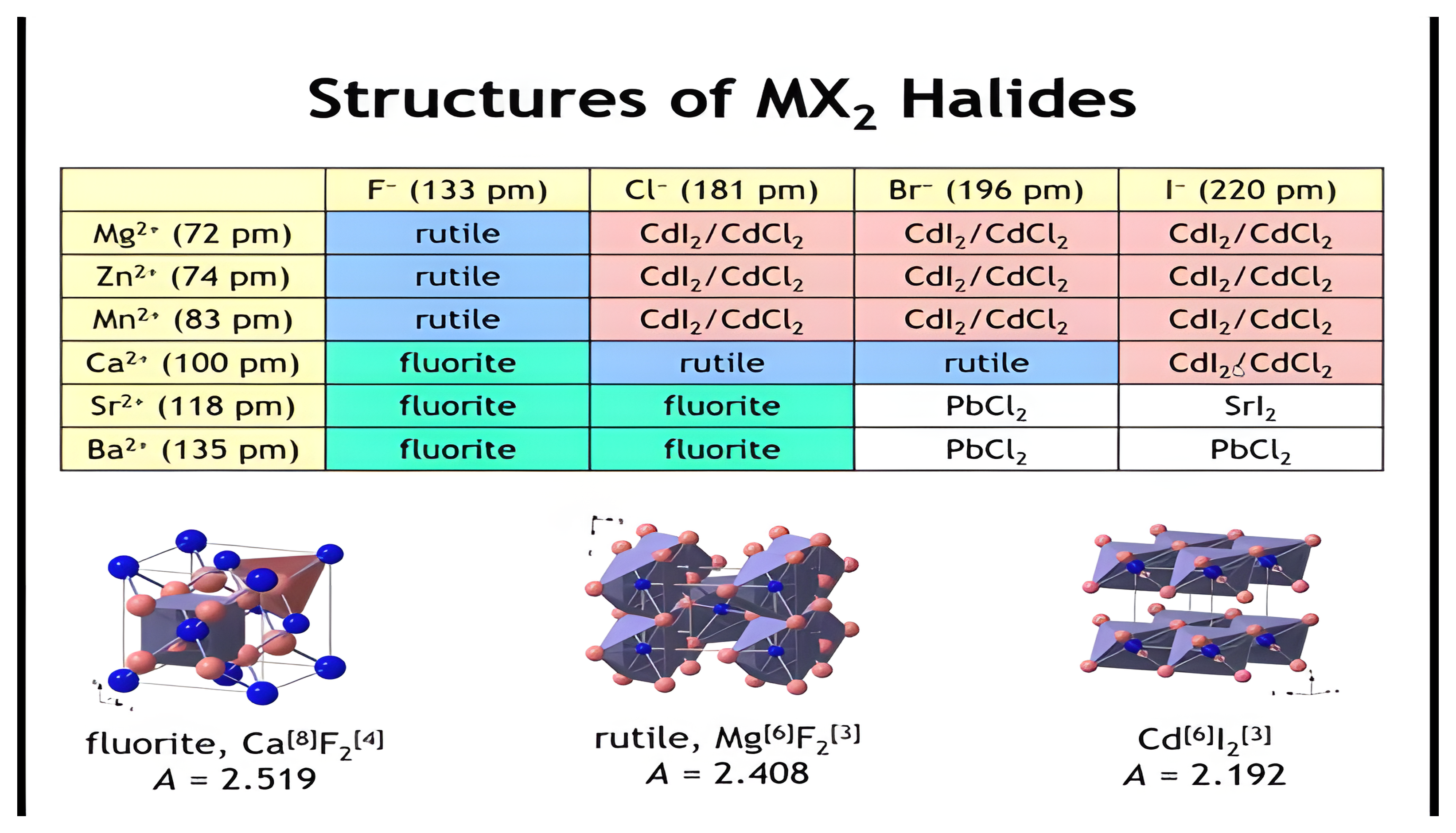
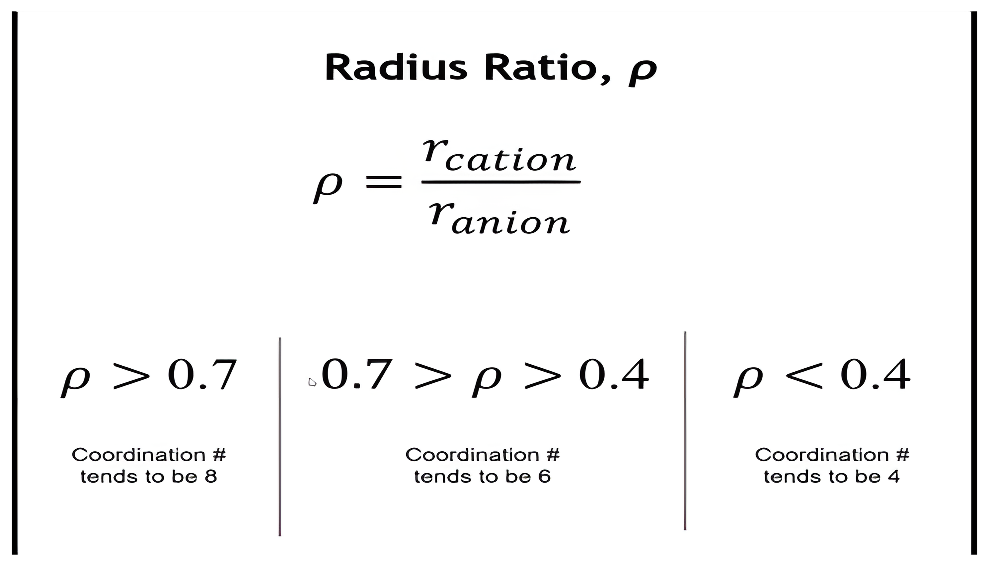
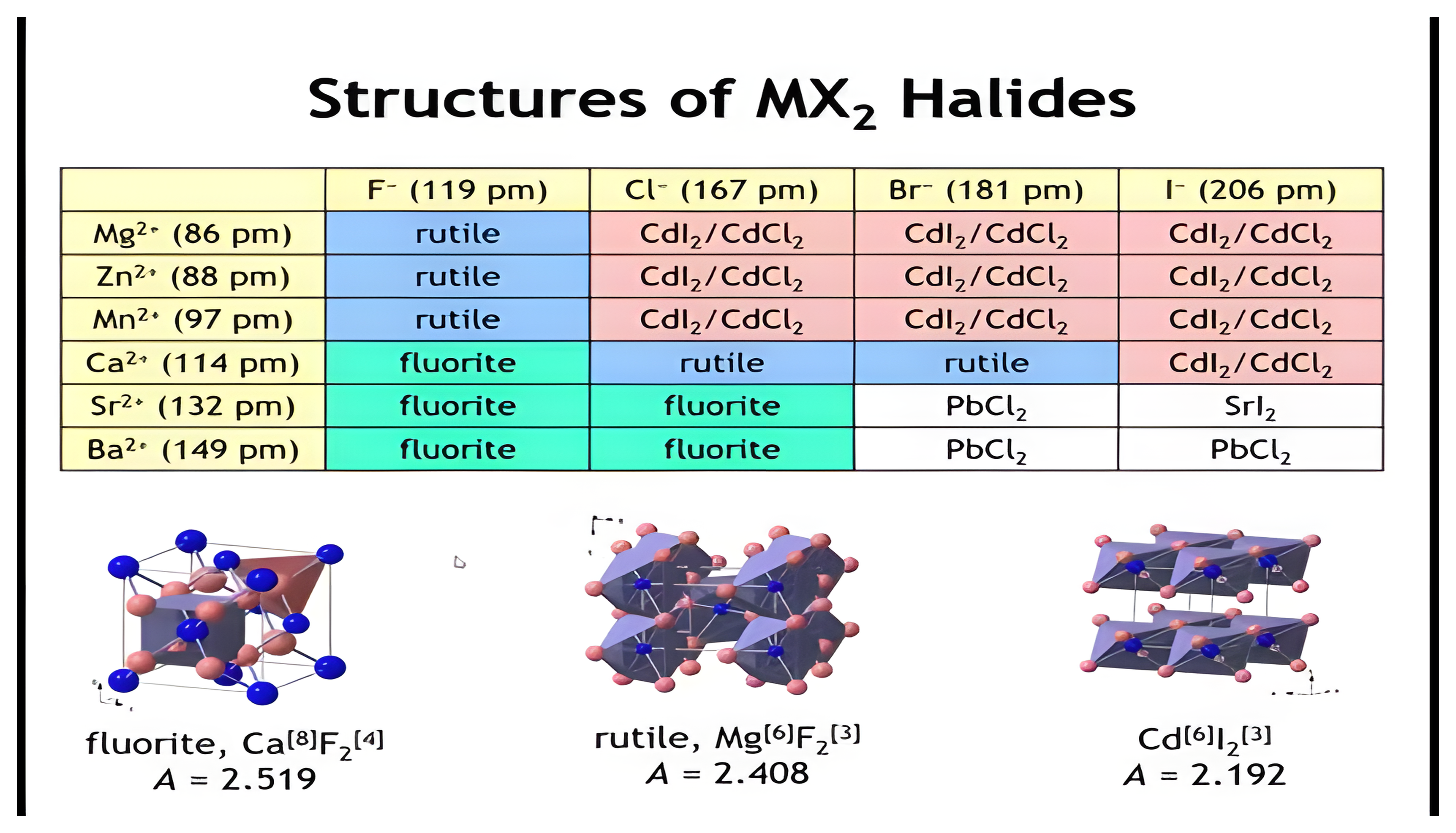
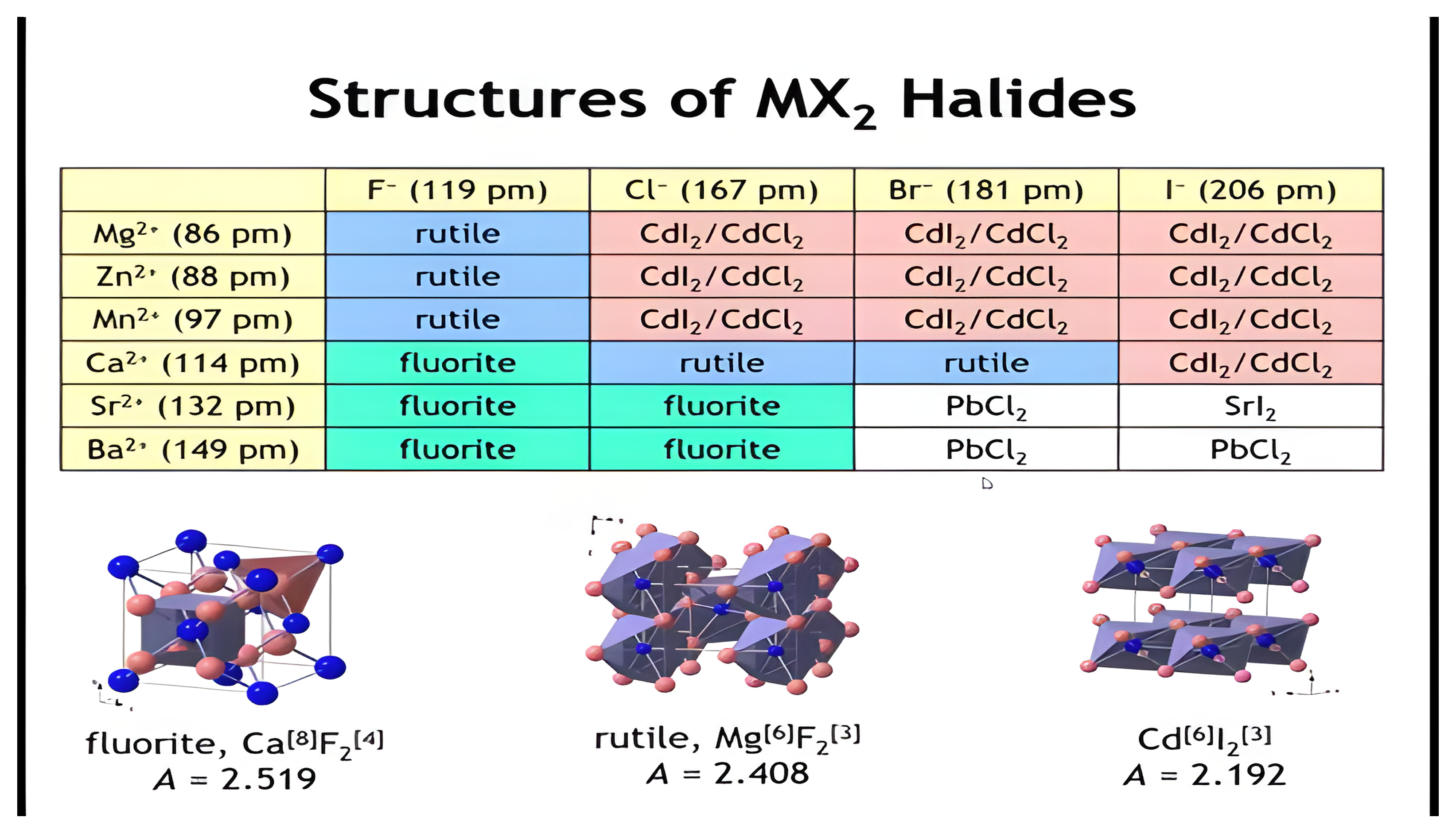
- Relate cation/anion size ratios to coordination number and stable crystal structures (fluorite, rutile, layered).
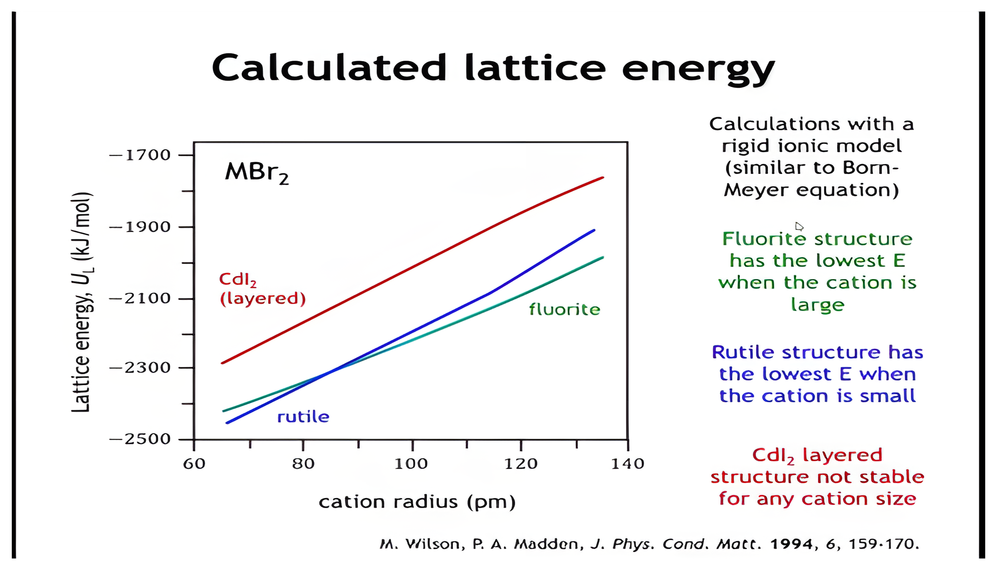
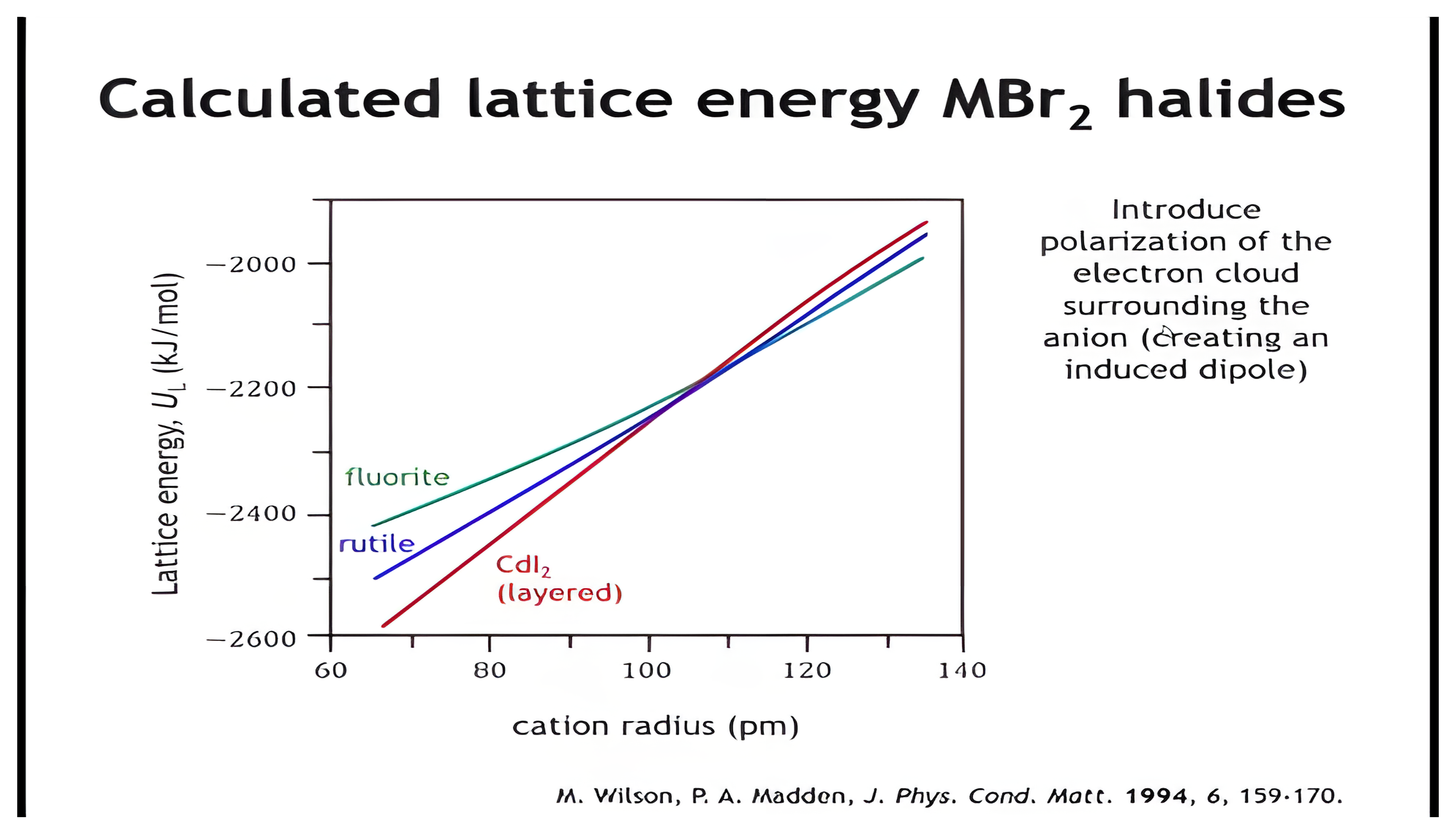
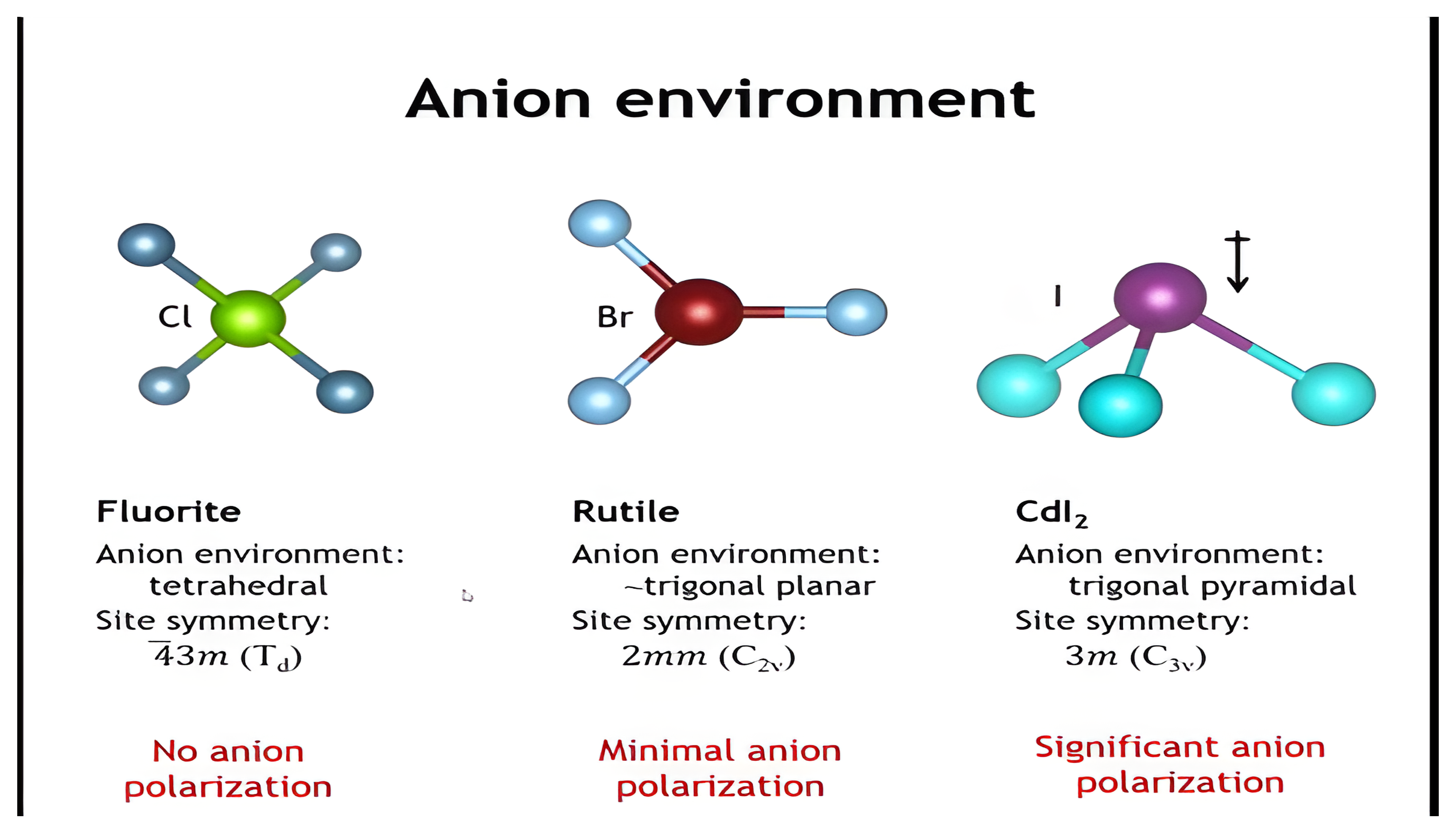
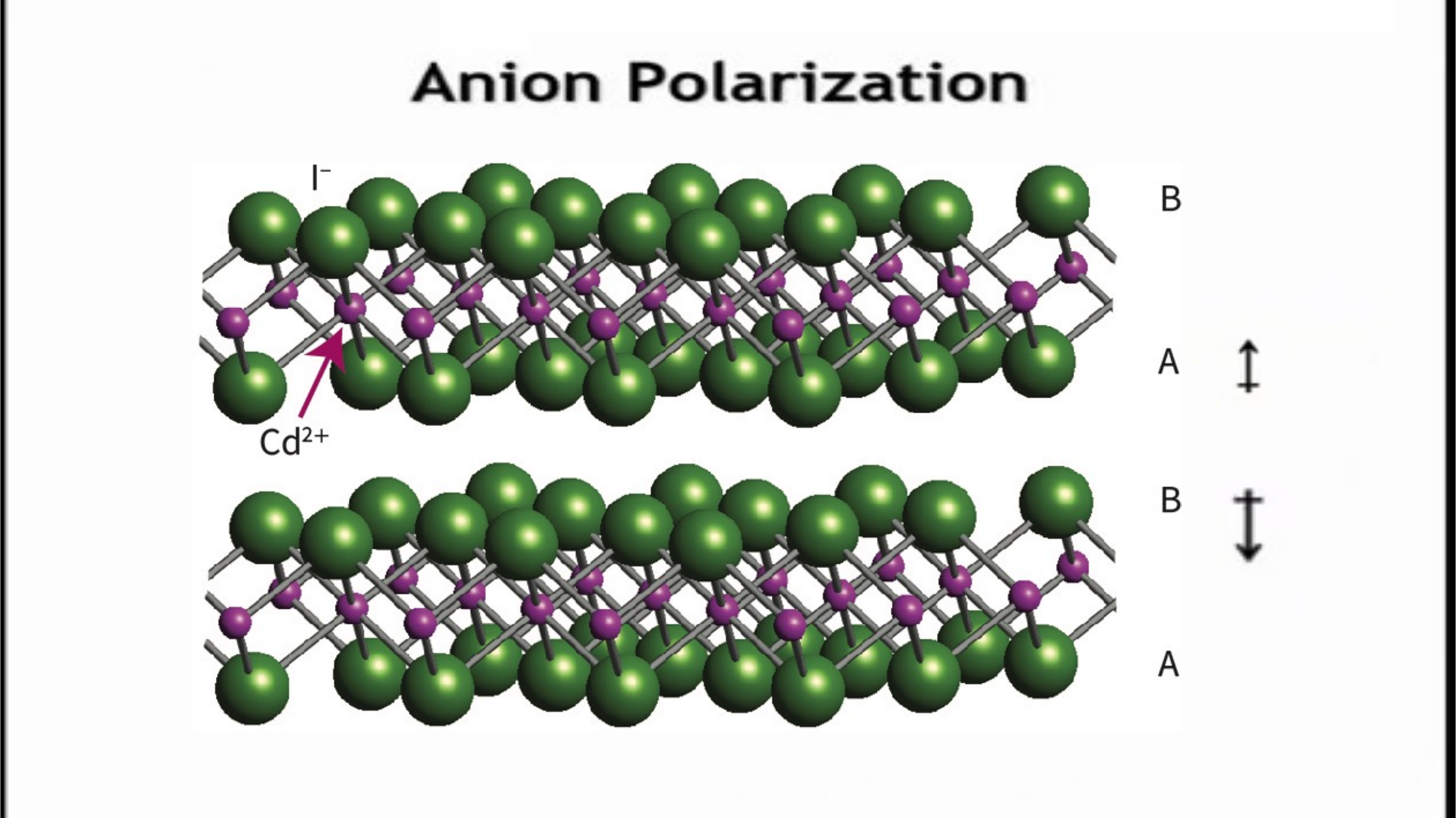
- Describe how anion polarizability and induced dipoles stabilize layered structures in heavier halides.
Complete Lattice Energy Expression
$U_L = -\frac{z_1 z_2 e^2 N_\mathrm{A}}{4πε_0 d_0}\,A\left(1-\frac{ρ}{d_0}\right)-\frac{N_\mathrm{A}C}{d_0^{\,6}}+2.25\,N_\mathrm{A}hυ_\mathrm{max}$
- [A] Coulomb energy
- [B] Repulsive interaction (9-17%)
- [C] Dispersion forces (0.1-5%)
- [D] Zero point energy (<1.5%)
| Substance | [A] kJ | [B] kJ | [C] kJ | [D] kJ |
|---|---|---|---|---|
| NaCl (U=−766) | −859 | 99 | −12 | 7 |
| MgO (U= −3921) | −4631 | 698 | −6 | 18 |
Summary
- Born–Mayer equation combines Coulomb attraction with a short-range repulsive term to approximate lattice energy.
- Example: For KCl, calculated lattice energy ≈ −679 kJ/mol vs. experimental −718 kJ/mol (Born–Haber).
- Shannon radii provide coordination-specific values to estimate d₀.
- The model systematically underestimates lattice energies by ~3–6%.
- Adding dispersion and zero-point energy terms improves accuracy slightly, but the main trend is well captured.
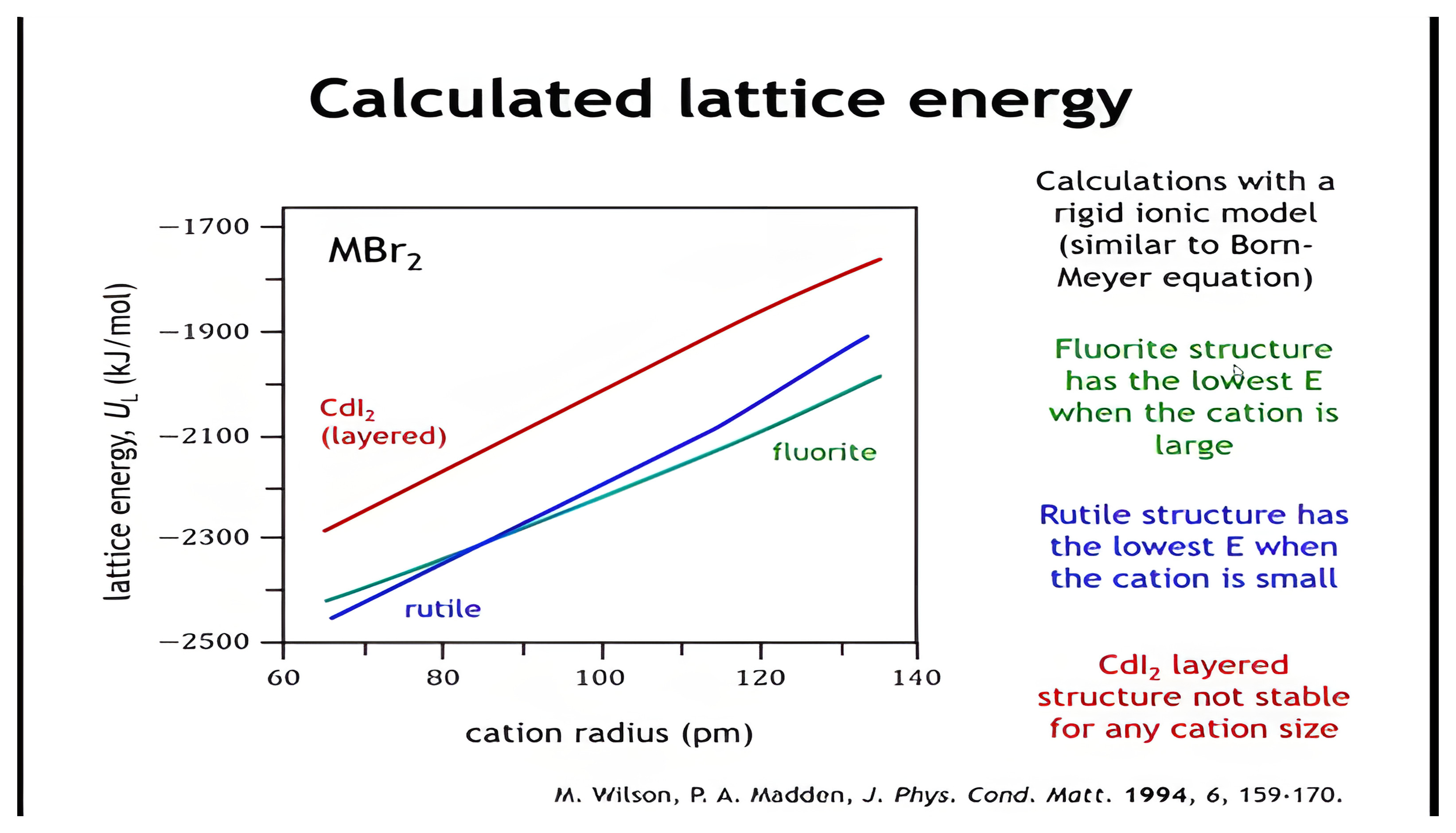
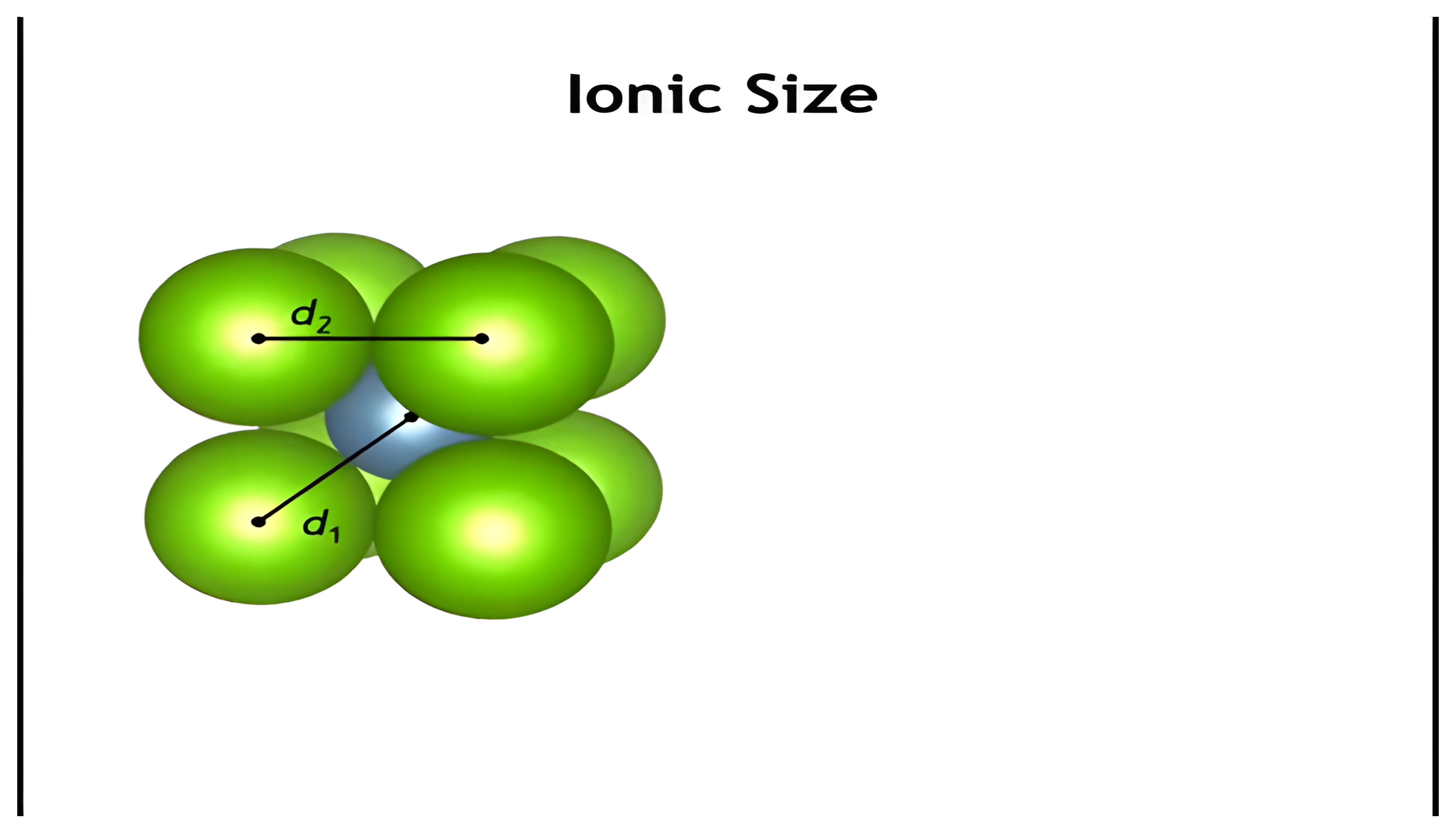
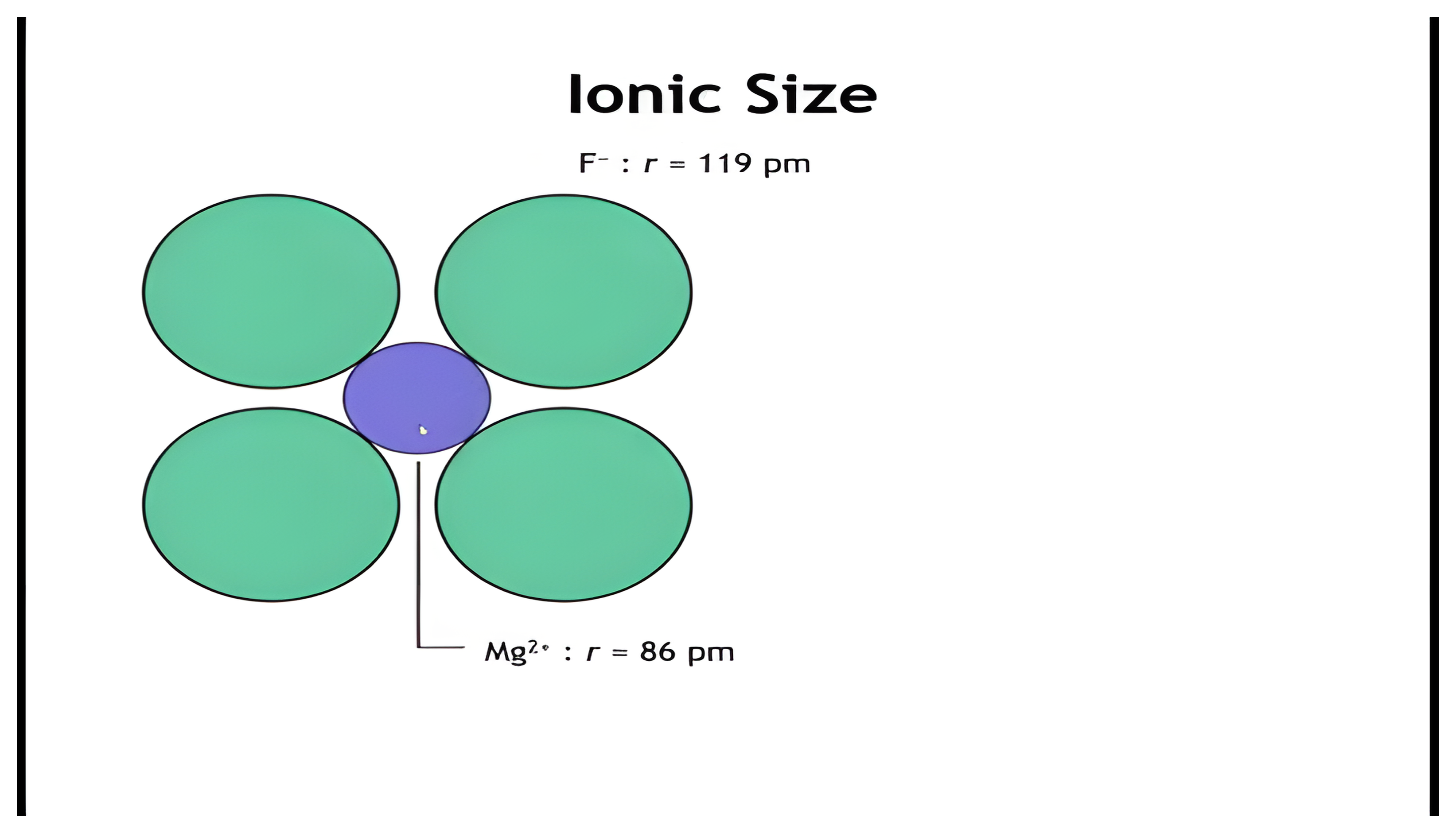
- Radius ratio rule: smaller cations (or larger anions) lower coordination numbers → 8 → 6 → 4.
- Structure stability trends:
- Large cations + small anions → fluorite (CN = 8).
- Small cations → rutile (CN = 6).
- Large, polarizable anions (Br⁻, I⁻) → layered CdI₂-type structures, stabilized by anion polarization.
- Symmetry of cation arrangement dictates whether polarization cancels (fluorite, rutile) or enhances stability (layered).
Homework
5.6 With the exception of helium, all noble gases solidify at low temperature. The lack of ionic or covalent bonding means that atoms are held together by dispersion forces alone. Given the melting points of the noble gases: Ne = 24 K, Ar = 84 K, Kr = 116 K, Xe = 161 K, what can you say about the strength of the London dispersion forces as the principal quantum number of the outermost shell increases? What is the explanation for this trend?
Practice questions
Work the Lecture 11 practice questions before the next class. They cover the free energy of mixing and the method of tangents, Coulomb interactions and the Madelung constant, the Born–Mayer lattice energy and the Born–Haber cycle, and radius ratios, anion polarization, and MX₂ structure choice.
Open the Lecture 11 practice questions
Every question carries a worked explanation, so you can check your reasoning as you go.